Aggregate Wind Power Models
In many cases, especially in the absence of transmission congestion, we are less concerned about the power from individual wind plants, and more concerned about the aggregate wind power. In these cases, we need not model the individual wind plants, and instead focus only on the aggregate wind power.
In this section we identify appropriate parametric models of the probability density functions of aggregate instantaneous wind power and wind power variation. Parametric approximation has several advantages including: fewer data points are needed to ‘‘fill out’’ the distribution; analytic calculations are more tractable; and the model can be expressed with fewer pieces of information— hopefully just one or two parameters.
Instantaneous Aggregate Wind Power Model
The shape of the histograms of aggregate wind power in Fig. 1 suggests that we seek a model with two parameters—one controlling the shape at low wind power, the other at high wind power.
One promising candidate is the Beta probability density function:
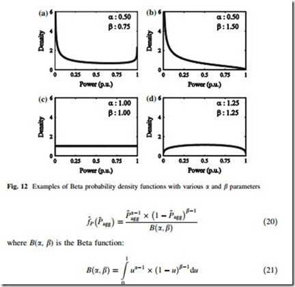
and a and b are shape parameters and u is the variable of integration. The domain of the Beta pdf is [0, 1], thereby necessitating the use of normalized aggregate wind power values. A wide range of shapes are possible by careful selection of a and b, as shown in Fig. 12.
Beta Distribution Parameter Selection
An important advantage of using the Beta pdf to model aggregate wind power is that its parameters lend themselves to meaningful interpretation [42]. Values of a that are less than 1 indicate an increasing probability density of 0 or near-zero power output; whereas a values greater than 1 indicate decreasing probability density over this range. The b values have a similar interpretation. If b is greater than 1, then the probability density decreases toward full power output; whereas if it is less than 1, there is increasing probability density.
In the absence of specific information, heuristic guides can be followed for modeling aggregate wind power. For low diversity, a and b are both greater than 1; for medium diversity a [ 1 and b \ 1; and for higher diversity a \ 1, b \ 1 or a Gaussian distribution can be used. Specific values for the parameters can be selected from estimations of the mean and variance.
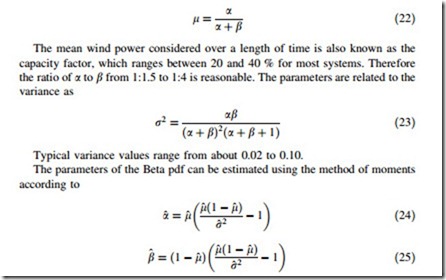
The shape parameters are related to the mean as
where l^ and r^2 are the sampled mean and variance of the wind power data. There is no closed-form MLE of ^a and b^, but numerical methods can be used to compute them [43].
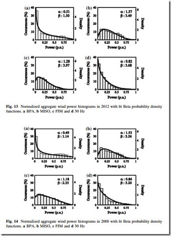
Traces of the Beta pdf with parameters fit using MLE to aggregate wind power data from four large systems in different years are found in Figs. 13 and 14. In each case the Beta pdf is able to reasonably approximate the data. A rigorous evaluation of the fit of Beta distributions to aggregate wind power is found in [42].
Aggregate Wind Power Variation Model
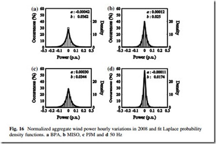
Wind speed and wind power tend to exhibit large autocorrelation coefficients at short time lags. As such DP~ tends to be near-zero, with only rare occurrences of extreme deviations. The trend is that of symmetric and exponential decay.
An appropriate distribution for these features is the Laplace distribution, also known as the double exponential distribution. The Laplace pdf is where DP~agg is normalized aggregation power output variation and a and b are the location and scale parameters, respectively. The scale parameter is an indicator of the variability, where a larger scale parameter indicates greater variability.
Laplace Distribution Parameter Selection
The parameters of the Laplace distribution can be fit using MLE method where ^a is equal to the sample median, which is usually zero, and ^b is computed from
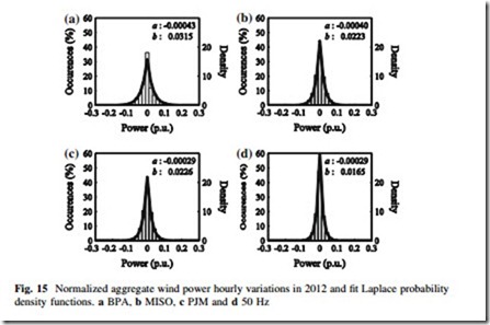
The scale parameter is generally between 0.015 and 0.04 for 1 h variation periods. The scale parameter tends to increase with longer variation periods. Traces of the Laplace pdf with parameters fit using MLE to hourly aggregate wind power variation data are found in Figs. 15 and 16. In each case the Laplace pdf is
able to reasonably approximate the data. A rigorous evaluation of the fit of Laplace distributions to aggregate wind power is found in [44].
Influence of Variation Period
An important factor influencing the pdf of wind power variation is the variation period. As discussed in Sect. 4.4, the variation in wind power from wind plants exhibits greater correlation as the variation period increases. Additionally, there is also more time for the wind power to change, so there is greater potential for extreme variation. Figure 17 shows histograms and fit Laplace pdfs for hourly and 4-hourly variation periods. It is clear that a longer variation period results in a broader distribution, and hence, more variability that must be managed. The Laplace distribution is able to reasonably fit the data at both variation periods mainly by adjusting its scale parameter.
