Perhaps one of the greatest opportunities to reduce operating expenses and enhance overall performance without investing additional effort is to first simulate the industrial processes and systems under control or to be controlled. In fact, most industrial control designs rely on simulation of the process and system, which allows the best control strategies and also the best process and system parameters for effective industrial control to be determined. Simulation studies also allow complex what-if scenarios to be viewed, which may be difficult with the real process and system.
However, it must always be borne in mind that any simulation results obtained are only as good as the model of the process or system that is used to obtain them. This does not mean that every effort should be made to get the model as realistic as possible, just that it should be sufficiently representative to produce good enough results.
Creating such a model of an industrial process or system, whatever its type and complexity, requires all features to be described in a form that can be analyzed.
Industrial processes can be classified as discrete or continuous. Industrial systems are embedded or distributed. A key problem in modeling and simulation lies in hybrid processes or systems which require special numerical procedures and integration algorithms. These advanced control strategies can be obtained by experimental approaches to the system and process modeling, so-called “process or system identification”. Additionally, the interplay between modeling and control has led to a wide variety of iterative modeling and control strategies, in which control-oriented identification is inter- leaved with control analysis and design, aiming at the gradual improvement of industrial process controller performance.
Two industrial simulation methods have been developed: computer-direct and numerical- computation. Computer-direct simulation is a fast and flexible tool for generating models, either for current systems where modifications are planned, or for completely new systems. Running the simulation predicts the effect of changing system parameters, provides information on the sensitivity of the system, and helps to identify an optimum solution for specific operating conditions. Numerical-computation simulation is the key to comprehending and controlling the full-scale industrial plant used in the chemical, oil, gas and electrical power industries. Simulation of these industrial processes uses the laws of physics and chemistry to produce mathematical equations to dynamically simulate all the most important unit operations found in process and power plants.
The most important topics to be addressed with respect to simulation routines include modeling and identification; control and simulation; simulators and tools.
MODELING AND IDENTIFICATION
Industrial control can be split into process and system control, which divides the modeling of industrial control into process modeling and system modeling accordingly.
Process modeling is the mathematical representation of a process by application of material properties and physical laws governing geometry, dynamics, heat and fluid flow, and so on, in order to predict its behavior. For example, finite element analyses are used to represent the application of forces (mechanics, strength of materials) on a defined part (geometry and material properties), and to model a metal forging operation. The result of the analyses is a time-based series of pictures, showing the distribution of stresses and strains, which depict the configuration and state of the part during and after forging. The behavior predicted by process models is compared with the results of actual processes to ensure that the models are correct. As differences between theoretical and actual behavior are resolved, the basic understanding of the process improves and future process decisions are more informed. The analysis can be used to iterate tooling designs and make processing decisions without incurring the high costs of physical prototyping.
System modeling is for a system typically composed of a number of networks that connect its different nodes, and where the networks are interconnected through gateways. One example of such a system is an automotive system that include a high-speed network (based on the controller area network) for connecting engine, transmission, and brake-related nodes; and one network for connecting other “body electronics functions” from instrument panels to alarms. Often, a separate network is available for diagnostics. A node typically includes sensor and actuator interfaces, a microcontroller, and a communication interface to the broadcast (analog or digital) bus. From a control function perspective, the vehicle can be controlled by a hierarchical system, where subfunctions interact with each other and through the vehicle dynamics to provide the desired control performance. The subfunctions are implemented in various nodes of the vehicle, but not always in a top-down fashion, because the development is strongly governed by aspects such as the organizational structure (internal organization, system integrators, and subcontractors).
Models and simulation features should form part of a larger toolset that supports the design of control systems to meet the main identified challenges: complexity, multidisciplinarity, and depend- ability. Some of the requirements of the models are as follows:
1. The developed system models should encompass both time- and event-triggered algorithms, as typified by discrete-time control and finite-state machines (hybrid systems).
2. The models must represent the basic mechanisms and algorithms that affect the overall system timing behavior.
3. The models should allow co-simulation of functionality, as implemented in a computer system, together with the controlled continuous time processes and the behavior of the computer system.
4. The models should support interdisciplinary design, thus taking into account different supporting methods, modeling views, abstractions and accuracy, as required by control, system, and computer engineers.
5. Preferably, the models should also be useful as a descriptive framework, visualizing different aspects of the system, as well as being useful for other types of analysis such as scheduling analysis.
19.1.1 Industrial process modeling
Any industrial process can be described by a model of that process. In terms of control requirements, the model must contain information that enables the prediction of the consequences of changing process operating conditions. Within this context, a process allows the effects of time and space to be scaled, and extraction of properties and hence simplification, to retain only those details relevant to the problem. The use of models, therefore, reduces the need for real experimentation, and facilitates the achievement of many different purposes at reduced cost, risk, and time.
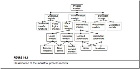
Depending on the task, different model types will be employed. Process models are categorized as shown in Figure 19.1.
(1) Mathematical models
As specified in Figure 19.1, mathematical models include all of the following:
(a) Mechanistic models
If a process and its characteristics are well defined, a set of differential equations can be used to describe its dynamic behavior. This is known as the development of mechanistic models. The mechanistic model is usually derived from the physics and chemistry governing the process. Depending on the system, the structure of the final model may either be a lumped parameter or a distributed parameter representation.
Lumped parameter models are described by ordinary differential equations, whereas distributed parameter systems representations require the use of partial differential equations. Nevertheless, a distributed model can be approximated by a series of ordinary differential equations and a set of simplifying assumptions. Both lumped and distributed parameter models can be further classified into linear or nonlinear descriptions. Usually nonlinear, the differential equations are often liberalized to enable tractable analysis.
In many cases, typically due to financial and time constraints, mechanistic model development may not be practically feasible. This is particularly true when knowledge about the process is initially vague, or if the process is so complex that the resulting equations cannot be solved. Under such circumstances, empirical or black-box models may be built, using data collected from the plant.
(b) Black box models
Black box models are simply the functional relationships between system inputs and system outputs. By implication, black box models are lumped together with parameter models. The parameters of these functions do not have any physical significance in terms of equivalence to process parameters such as heat or mass transfer coefficients, reaction kinetics, and so on. This is the disadvantage of black box models compared to mechanistic models. However, if the aim is to merely represent faithfully some trends in process behavior, then the black box modeling approach is very effective.
As shown in Figure 19.1, black box models can be further classified into linear and nonlinear forms. In the linear category, transfer function and time series models predominate. Given the relevant data, a variety of techniques may be used to identify the parameters of linear black box models. Least- squares-based algorithms are, however, the technique most commonly used. Within the nonlinear category, time-series features are found together with neural-network-based models. The parameters of the functions are still linear and thus facilitate identification using least-squares-based techniques. The use of neural networks in model building has increased with the availability of cheap computing power and certain powerful theoretical results.
(2) Qualitative models
There are some cases in which the nature of the process may preclude mathematical description, for example, when the process is operated in distinct operating regions or when physical limits exist. This results in discontinuities that are not amenable to mathematical descriptions. In this case, qualitative models can be formulated. The simplest form of a qualitative model is the rule-based model that makes use of IF THEN ELSE constructs to describe process behavior. These rules are elicited from human experts. Alternatively, genetic algorithms and rule induction techniques can be applied to process data to generate these descriptive rules. More sophisticated approaches make use of qualitative physics theory and its variants. These latter methods aim to rectify the disadvantages of purely rule-based models by invoking some form of algebra so that the preciseness of mathematical modeling approaches can be achieved.
Of these, qualitative transfer functions appear to be the most suitable for process monitoring and control applications, which retain many of the qualities of quantitative transfer functions that describe the relationship between an input and an output variable, particularly the ability to embody temporal aspects of process behavior. The technique was conceived for applications in the process control domain. Cast within an object framework, a model is built up of smaller subsystems and connected together as in a directed graph. Each node in the graph represents a variable while the arcs that connect the nodes describe the influence or relationship between the nodes. Overall system behavior is derived by traversing the graph, from input sources to output sinks.
Fuzzy logic can also be used to build qualitative models. Fuzzy logic theory contains a set of linguistics that facilitates descriptions of complex and ill-defined systems. The magnitudes of changes are quantized as negative medium, positive large, and so on. Fuzzy models are used in everyday life without our being aware of their presence; in for example, washing machines, autofocus cameras, and so on.
(3) Statistical models
Describing processes in statistical terms is another modeling technique. Time-series analysis that has a heavy statistical bias may be considered to fall into this category. Statistical models do not capture system dynamics, but in modern control practice, they play an important role, particularly in assisting in higher-level decision making, process monitoring, data analysis, and, obviously, in statistical process control.
Given its widespread and interchangeable use in the development of deterministic as well as stochastic digital control algorithms, the statistical approach is made necessary by the uncertainties surrounding some process systems. This technique has roots in statistical data analysis, information theory, games theory, and the theory of decision systems.
Probabilistic models are characterized by the probability density functions of the variables. The most common is the normal distribution, which provides information about the likelihood of a variable taking on certain values. Multivariate probability density functions can also be formulated, but interpretation becomes difficult when more than two variables are considered. Correlation models arise by quantifying the degree of similarity between two variables by monitoring their variations. This is again quite a commonly used technique, and is implicit when associations between variables are analyzed using regression techniques.
Industrial system modeling
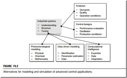
Modeling has been an essential part of industrial control since the 1970s. However, industrial control requires accurate models that are not easy to build. As a compromise, both data-driven modeling and computational intelligence provide additional modeling alternatives for advanced industrial control applications. These alternatives are illustrated in Figure 19.2.
(1) Phenomenological modeling approaches
Phenomenological modeling approaches aid in the construction and analysis of models whose ultimate purpose is to provide insights into system performance and improve understanding of how cooperative phenomena can be manipulated for the accomplishment of design strategies that increase the complexity of systems. Following the fundamentals which guide the structuring of the model, the system tasks are decomposed into the relevant phases and physicochemical phenomena involved, identifying the connections and influences among them and evaluating the individual rates. The clarification of rate-limiting phenomena is finally achieved by diverse strategies derived from dealing with the manipulation of driving forces. Empirical models are mostly used for phenomenological modeling to develop a control system. The structure and parameters do not necessarily have any physical significance, and, therefore, these models cannot directly be adapted to different production conditions.
(2) Data-driven modeling approaches
Data-driven modeling approaches are based on general function estimators of a black-box structure, which should capture correctly the dynamics and nonlinearity of the system. The identification procedure, which consists of estimating the parameters of the model, is quite straightforward and easy if appropriate data are available. Essentially, system identification means adjusting parameters within a given model until its output coincides as well as possible with the measured output of the real system. Validation is needed to evaluate the performance of the model.
The generic data-driven modeling procedure consists of the following three steps. The objective of the first step is to define an optimal plant operation mode by performing a model and control analysis. Basic system information, including the operating window and characteristic disturbances, as well as fundamental knowledge of the control structure, such as degrees of freedom of and interactions between basic control loops, will be obtained. The second step identifies a predictive model using data- driven approaches. A suitable model structure will be proposed based on the process dynamics extracted from the operating data, followed by parameter estimation using multivariate statistical techniques. The dynamic partial least squares approach solves the issue of autocorrelation. However, a large number of lagged variables are often required, which might lead to poorly conditioned data matrices. Subspace model identification approaches are suitable to derive a parsimonious model by projecting original process data onto a lower-dimension space that is statistically significant. If a linear model is not sufficient due to strong nonlinearities, neural networks provide a possible solution. The third step is model validation. Independent operating data sets are used to verify the prediction ability of the derived model.
(3) Intelligent modeling methods
Intelligent methods are based on techniques inspired by biological systems and human intelligence, for instance, natural language, neural network rules, semantic network rules, and qualitative models. Most of these techniques have already been used in conventional expert systems.
Computational intelligence can provide additional tools, since humans can handle complex tasks including significant uncertainty on the basis of imprecise and qualitative knowledge. Computational intelligence is the study of the design of intelligent agents. An agent is something that acts in, and affects its environment. They include worms, dogs, thermostats, airplanes, humans, organizations, and society, and so on. An intelligent agent is a system that acts intelligently: what it does is appropriate to its circumstances and its goal; it is flexible to changing environments and changing goals; it learns from experience; and it makes appropriate choices given perceptual limitations and finite computation. The central goal of computational intelligence is to understand the principles that make intelligent behavior possible, in natural or artificial systems. The main hypothesis is that reasoning is compu- tation. The central engineering goal is to specify methods for the design of useful, intelligent artifacts.
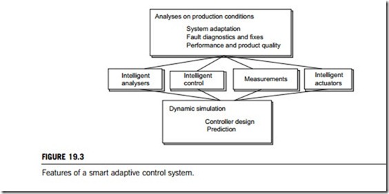
Modeling is also used on other levels of advanced control: high-level control is in many cases based on modeling operator actions, and helps to develop intelligent analyzers and software sensors. The products of modeling are models that are used in adaptive and direct model-based control. Smart adaptive control systems integrate all these features, as shown in Figure 19.3.
Adaptive controllers generally contain two extra components compared to standard controllers. The first is a process monitor, which detects changes in process characteristics either by performance measurement or by parameter estimatation. The second is the adaptation mechanism, which updates the controller parameters. In normal operation, efficient reuse of controllers developed for different operating conditions is good operating practice, as the adaptation always takes time.
An adaptation controller is a controller with adjustable parameters, that can perform online adaptation. However, controllers should also be able to adapt to changing operating conditions in processes where the changes are too fast or too complicated for online adaptation. Therefore, the area of adaptation must be expanded; the adaptation mechanism can be either online or predefined.
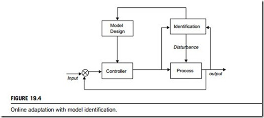
This includes self-tuning, auto-tuning, and self-organization. For online adaptation, changes in process characteristics can be detected through online identification of the system model, or by assessment of the control response, that is, performance analyses. The choice of measure depends on the type of response the control system designer wishes to achieve. Alternative measures include overshoot, rise time, setting time, delay ratio, frequency of oscillations, gain and phase margins, and various error signals.
The identification block typically contains some kind of recursive estimation algorithm that aims at the current instant. Figure 19.4 shows online adaptation with model identification. The model can be a transfer function, a discrete-time linear model, a fuzzy model, or a linguistic equation model. Adaptation mechanisms rely on parameter estimations of the process model: gain, dead time, time constants etc.
Classic adaptation schemes do not cope easily with large and fast changes unless the adaptation rate is very high. This is not always possible: some a priori knowledge about the dynamic behavior of a plant or factory may be necessary. One alternative for these cases is a switching control scheme that selects a controller from a finite set of predefined fixed controllers. Multiple-model adaptive control is hence classified as mode-based control. Intelligent methods provide additional techniques for online adaptation. Fuzzy, self-organizing controllers give an example of intelligent modeling methodologies. Another example of this approach is a meta-rule approach, in which parameters of a low-level controller are changed by a meta-rule supervisory system whose decisions are based on the perfor- mance of the low-level controller. Meta-rule modules consist typically of a fuzzy rule base that describes the actions needed to improve the low-level fuzzy logic controller.
(2) Predefined adaptation
This is becoming more popular as modeling and simulation techniques improve. Gain scheduling, including fuzzy-gain scheduling and linguistic-equation-based gain scheduling, provides a gradual adaptation technique for a fixed control structure. Predefined adaptation uses very detailed models; for example, distributed parameter models can be used to tune adaptation models of a solar-powered plant. The resulting adaptation models or mechanisms should be able to handle special situations in real time without using detailed simulation models.
Predefined actions adapt rapidly enough to remove the need for online identification, or for classic mechanisms based on performance analysis. In these cases, the controller could be classified as a linguistic equation based on gain scheduling. The adaptation model is generated from the local tuning results, but the directions of interactions are usually consistent with process knowledge.
Identification for model-based control
Process control systems typically include one or more controllers which are communicatively coupled to each other, to at least one host or operator workstation and to one or more field devices via analog, digital or combined buses. Some systems use function blocks or groups of function blocks, referred to as modules to perform control operations.
Industrial process controllers are typically programmed to execute different algorithms, routines or control loops for a process, such as flow, temperature, pressure, or level control loops. Generally speaking, each loop includes one or more input blocks, such as an analog-input, a single-output, or a fuzzy logic control function block, and an output block.
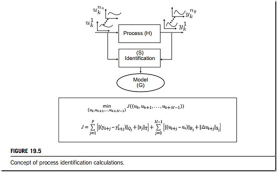
An identification experiment consists of perturbing process or system inputs and observing the responses from the outputs. A model describing this dynamic input-output relationship can then be identified directly by modifying variables and parameters. In a process or system control context, the end-use of such a model would typically be for designing industrial controllers. Ideally, the design of a control-oriented identification procedure could then be formulated by choosing a performance objective, then designing the identification in such a way that the performance achieved by the model- based controller on the true system is as high as possible. Figure 19.4 illustrates this procedure.
In the rest of this subsection, model-based identification for control is introduced very briefly; the mathematical, statistical and physical theories involved in this identification is beyond the scope of this book.
(1) Experiment design
Assuming you need to perform an identification, the first step is to design one or more experiments to capture the process’s dynamic behavior. To provide the best results, these experiments must satisfy the following criteria: all modes of process behavior must be represented in the measured data; transient and steady-state behavior must be represented from input to output; the experiments must not damage the plant or cause it to malfunction.
In many cases, such experiments can only be performed on a plant that is in operation. A controller might even be driving the plant (presumably one that is inadequate in some way). The experiment for this type of process would involve adding perturbation signals at the input and measuring the plant’s response to the controller’s command plus the perturbation.
It is important to remember that such experiments are generally used to develop linear plant models. Input signals must be chosen so the plant behavior remains (at least approximately) linear, meaning that the amplitude of the input signal (and possibly its rate of change) must be limited to a range in which the plant response is approximately linear. However, the amplitude of the driving signal must also be large enough so that corrupting effects such as noise and quantization in the measured output signal are minimized relative to the expected response.
(2) Data collection
The sampling rate for recording input and output data must be high enough to retain all frequencies of interest in the results. According to the Nyquist sampling theorem, the sampling rate (samples per second) must be at least twice the highest frequency of interest to enable reconstruction of the original signal. In practice, the sampling rate must be a little higher than this limit to ensure the resulting data will be useful. For example, if the highest frequency of interest was 20 Hz (hertz), a sampling rate of 50 Hz might be sufficient.
It is also important to keep corrupting effects such as noise and quantization to a minimum relative to the measured signals. The amplitudes of input signals must be sufficient to give large outputs relative to noise and quantization effects. This requirement must be balanced against the need to maintain the system in an approximately linear mode of operation, which typically requires that the input signal amplitudes be small.
(3) Identification calculations
Figure 19.5 gives the basic concept for model-based identification calculations. First, you must have
The situation described in the above shows that control-relevant models are obtained when identification takes place when a controller is already part of the process. As this controller is unknown before the model is identified, an iterative scheme is required to arrive at the desired situation: (1) perform an identification experiment with the process being controlled by an initial stabilizing controller; (2) identify a model with a control-relevant criterion; (3) design a model-based controller; (4) implement the controller in the process and return to the first step while using the new controller.
A motivation for applying an iterative scheme is the fact that when designing control systems, the performance limitations are generally not known beforehand. Therefore, a sketched iterative scheme can also be considered to allow improvement of the performance specifications of the controlled system as one learns about the system through dedicated experiments. In this way, improved knowledge of the process dynamics allows the design of a controller with higher performance, thus enhancing overall control performance.
