Model for Time-Varying Variables Representation
The proposed model consists in representing the w time-varying variables v1,v2,…,vw by one single random variable VT in the simulation process and to adopt a multiple states Markov model to represent it. Each state of this variable corresponds to one combination of states of the time-varying variables, and therefore the state of each one can be written as a function of VT by (9):
where Fv1, Fv2,…,Fvw are functions that map v1,v2,…,vw from VT.
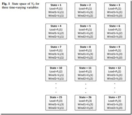
For example, considering three time-varying variables Load (PL), Wind1 (V1) and Wind2 (V2) that can be individually represented by three different states, a Markov model of 27 states for VT may be constructed where each state corresponds to one of the possible combinations of PL, V1 e V2, as shown in Fig. 1.
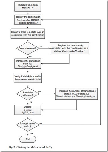
To enhance the efficient of the model for application to any number of time-varying variables, the time series are clustered into the most representative states in order to prevent that a large number of states is required to represent VT. However, this is not a requirement of the model and it could be used without any clustering. The k-means technique is used to perform the statistical clustering of the time series, but other techniques may be used as well [13]. Thus, based on the w clustered time series v1c,v2c,…,vwc, the Markov model for VT is obtained by the algorithm shown in Fig. 2.
After applying this algorithm, a Markov model of VT with NT states is available, similar to the one shown in Fig. 1, where each state of VT represents a unique combination of the time-varying variables v1c,v2c,…,vwc.
From this model, the transition rates between the states of VT may be calculated and then used to obtain the transition intensity matrix A [14] that is used to calculate the stead state probabilities of each state of VT. Having the steady state probabilities of all states of VT, sampling a state is done by applying the IT method to the CDF of VT in a similar way as described for the independent components. From generating a random number Uk uniformly distributed between [0, 1], the state of VT is obtained by (10), where Pi = P(VT B i).
The conceptual algorithm for composite reliability evaluation by nonsequential MCS considering correlated time-varying variables is shown below:
(1) Sample the state of each independent component by (3);
(2) Sample the state of VT by (10);
(3) Identify the state of each time-varying variable by (9);
(4) Configure the system state x based on the sampled states of the independent components and the time-varying variables;
(5) Calculate the value of the test functions F(x) that are defined for evaluating each reliability index;
(6) Update the reliability indices estimates EðFÞ based on the results of step 5;
(7) If the coefficients of variation of the indices (a) are less than an acceptable tolerance, stop the simulation; otherwise, return to step 1.
The main reliability indices calculated in nonsequential simulation for composite generation and transmission systems are the loss of load probability (LOLP, %), the expected power not supplied (EPNS, MW) and the loss of load frequency (LOLF) (occurrences). From these indices, others may be derived, such as the expected energy not supplied (EENS, MW h), the loss of load duration (LOLD, h), etc.


