Individual Wind Plant Model
The characteristics of aggregate wind power—especially at low levels of geo- graphic diversity—depend on the characteristics of the system’s constituent wind plants. We first derive an analytic model of wind plant power output under ide- alized conditions: that the wind speed follows a parametric probability density function and the energy conversion process is deterministic, among other assumptions. We conclude the section by considering non-idealities in wind plant power production.
The power delivered by a wind plant Pi is the sum of the real power produced by its constituent wind turbines, less collector system losses:
where M is the number of wind turbines in the wind plant, PWT, j is the real power generated by the jth wind turbine and PL,i is the ith wind plant’s collector system losses at the current operating state.
Although (1) appears straightforward, wind turbines are nonlinear energy conversion devices whose power output is primarily dependent on wind speed, which is a random variable. This implies that Pi will be stochastic, and that a probabilistic model of Pi can be derived by transforming the probability density function of the wind speed.
Probabilistic Wind Speed Model
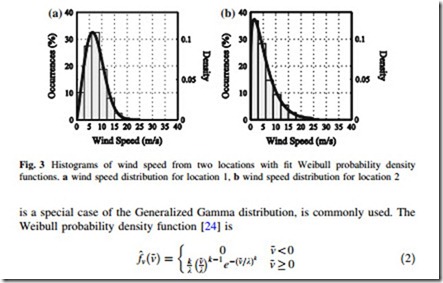
Let ~v be a random variable representing the wind speed at a certain wind turbine with corresponding probability density function fvð~vÞ. The presence of the tilde indicates that the variable is random. We can approximate fvð~vÞ by the repeated independent sampling of ~v. These samples can be binned into a histogram and scaled to approximate fvð~vÞ. Two typical, yet specific, scaled histograms of wind speed are shown in Fig. 3.
Although histograms are helpful visual approximations of probability density functions, it is often desirable to represent them using a parametric function. Let ^fvð~v; hÞ be the model of fvð~vÞ with parameters arranged in the vector H. For the sake of brevity, we will suppress H in all distributions hereafter, so that, for
example, ^fvð~vÞ represents the parametric model of fvð~vÞ.
Returning to Fig. 3, we see that each histogram is asymmetric with a distinctly
positive skewness, indicating that high wind speeds are less frequent than low wind speeds. These characteristics can be modeled using the three-parameter Generalized Gamma distribution [23]. However, estimating the parameters of this distribution can be difficult. Instead, the two-parameter Weibull distribution, which
where k and k are the shape and scale parameters, respectively. The parameters can be estimated from sampled data using the maximum likelihood estimation (MLE) method or the method of moments, though for the Weibull distribution these methods can be mathematically cumbersome [25, 26]. Examples of Weibull distributions with parameters estimated using MLE are shown as the solid traces in Fig. 3. In each case, the parametric function is a reasonable approximation to the data.
The two-parameter Weibull model can often be simplified to a single parameter model without appreciably sacrificing accuracy. For locations with wind regimes suitable for wind plant development, the estimated shape parameter of the Weibull distribution is often near 2.0. Therefore, the Weibull distribution can be reduced to the Rayleigh distribution [24]. A useful feature of the Rayleigh distribution is that its parameter can be estimated with the method of moments using only the mean of the wind speed, which is sometimes the only quantity available.
Idealized Wind Turbine Power Curve
We next examine the effect of the wind turbine in shaping the wind power probability density function. Wind turbines convert a portion of the kinetic energy into a mass of moving air to electrical energy by way of electric generator. The electrical power output by a wind turbine is computed from:
where Cp is the dimensionless power coefficient, A is the area swept by the rotor blades in m2, and q and ~v are the density and velocity of the air mass incident to the wind turbine, in kg/m3 and m/s, respectively [27]. The power coefficient represents the overall efficiency of the energy conversion process, which depends on turbine design and operating state. If a constant Cp can be maintained, then the wind speed and wind power are cubically related. Under low or high wind speed conditions the wind turbine is operated such that Cp is zero, for reasons discussed later. Although (3) is useful, a more common and illustrative way to show the relationship between wind speed and wind turbine power output is with the power curve.
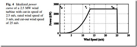
A power curve deterministically maps each wind speed to the corresponding power output of a wind turbine. An example of an idealized power curve is shown in Fig. 4. In general, there are four regions of operation.
At low wind speeds no electrical power is produced and Cp is zero. The power in the wind is not enough to either overcome the friction of the drivetrain, or to result in positive net power production. The threshold wind speed at which power generation begins is known as the cut-in wind speed (vci).
Between Cut-in and Rated Wind Speed ðvci ::; v\vr Þ
When the wind speed is between the cut-in and rated wind speed (vr), the wind turbine generates power. In this region, the turbine is designed or controlled to maximize Cp, and a nearly cubic wind speed-turbine power relationship is observed. This relationship can be approximated as At wind speeds above rated and below cut-out (vco), the wind turbine is controlled to maintain constant power production. As the wind speed increases over this region constant power is maintained by reducing Cp through active pitch control or passive stall design.
At and Above Cut-out Wind Speed ðvco ::; vÞ
At excessively high wind speeds, the wind turbine is in danger of mechanical failure. The turbine is aerodynamically slowed and stopped, and then mechanically locked into place to prevent rotation. Cp is zero over this region.
The effect of the varying power coefficient can be implicitly accounted for by expressing (3) as the piecewise function PWT = g(v), where g(v):
As previously mentioned, the power curve in Fig. 4 and expressed as (5) are idealized. Most utility-scale wind turbine manufacturers develop the power curve for a particular wind turbine model under carefully controlled conditions according to accepted standards [28]. Field performance of wind turbines can be inconsistent and appreciably differ from the manufacturer-supplied power curve. These non- idealities are discussed in detail in Sect. 3.4.
Idealized Wind Plant Model
A basic model of power from a wind plant is
where P~i is the total real power from the M wind turbines of wind plant i. This model makes several assumptions, such as all wind turbines experience the same wind speed and have the same power curve. We will discuss the reasonableness of these assumptions in Sect. 3.4. However, for the following, we will assume that (6) holds. Since P~i is a random variable, we can characterize it with a probability density function or cumulative distribution function (cdf).
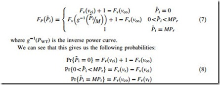
Let the cdf of the wind speed be Fvð~vÞ and let the cdf of the wind power from the wind plant be FP P~i . The cdf of the power from the wind plant is the piecewise function:
As there is a measurable probability of wind power being exactly equal to either 0 or MPr, we do not have a purely continuous distribution function. We instead have a mixed discrete/continuous distribution function.
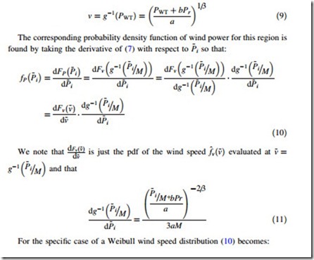
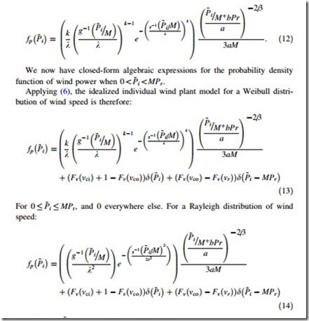
Our pdf for wind power, then, will need to use the Dirac delta function dð·Þ to address the probabilities of wind power being exactly equal to either 0 or MPr. For all other values of wind power, we can calculate the pdf using the traditional change-of-variables method. Using (5), the inverse power curve for the region between 0 and MPr is
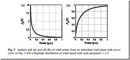
The models of individual wind plant power output in (13) and (14) were analytically derived and are dependent only on a small number of wind speed and power curve parameters. Figure 5 shows an example of the pdf and cdf of a wind plant. We note that the pdf shown is similar in appearance to that of Fig. 1a, which is reassuring. However, there are differences, particularly near rated power. Our analytic model overestimates the probability of rated power production from the wind plant. This discrepancy is an artifact of the idealized assumptions implied by (6). Despite the differences the derived model has utility—it serves as a reasonable starting point in the absence of additional data, and it allows for further analytic manipulation, as we will see later.
Non-idealized Wind Plant Modeling
The derived probability density functions in (14) and (15) are idealized models of wind power under several assumptions implied by (6), including:
1. the collector system is lossless;
2. all wind turbines are in service;
3. the power curves are deterministic for each wind turbine;
4. the wind speed and air density are the same at each wind turbine.
The first and second assumptions allow the wind plant to reach 100 % rated output. However, collector system losses are nonzero—usually between 1 and 5 % [29]—and wind turbines are routinely taken out of service due to scheduled maintenance or malfunction. A typical wind turbine requires regularly scheduled maintenance at 6 month intervals, although online condition monitoring may yield more optimal schedules [30]. Maintenance and malfunction-related outages can last several hours or longer, with offshore wind turbines generally requiring longer outages. For these reasons, a large wind plant may have one or more wind turbines out of service at any given time. Although rated power is not achieved, occurrences of near rated power may be common, as shown in Fig. 1a.
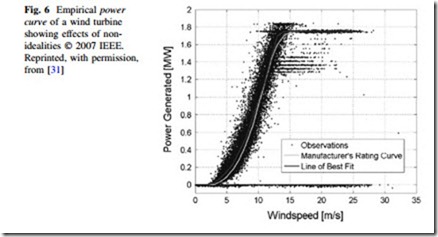
The third assumption, while greatly simplifying the model, is not substantiated by empirical data. Even after correcting for air density, power production strays from the manufacturer-supplied power curve for several reasons, including: dependency of power output on wind direction; forced curtailment; wind shear and turbulence; manufacturing and installation defects; efficiency degradation over time; and internal power consumption for control systems, lighting, pumps, and other functions. These effects are illustrated by an empirical power curve. An empirical power curve is constructed by plotting repeated in situ simultaneous measurements of wind speed and wind power, as shown in Fig. 6. It is clear from this figure that the idealized power curve model in (5) does not capture the true in situ relationship between wind speed and wind power.
The fourth assumption implied by (6) is naïve, though often used. In reality, wind turbines can be separated by several kilometres and installed in varying terrain. The wind turbines almost never simultaneously experience the same wind speed. In other words, there is geographic diversity within each wind plant that must be accounted for. Over the years, several approaches to more realistically account for non-idealities in power curves have been proposed [32–34]. Some involve creating sub-groups of wind turbines, where each sub-group has its own wind speed. Other methods involve creating data-driven wind plant power curves using statistical methods. Provided they are well-defined, wind plant power curves can be used in place of (5) to analytically derive a probabilistic model of wind power using the same steps detailed in Sect. 3.3.
To summarize our progress, we started by identifying suitable parametric probabilistic models of wind speed: Rayleigh or Weibull. We then developed pdfs and cdfs for individual wind plant power output by transforming the wind speed models using an idealized power curve, as in (13) and (14). This method can be used to account for non-idealities using a wind plant power curve if desired. We are now poised to consider the aggregate power production from a fleet of wind plants in a common system. To do this, we must model the correlation and dependency of wind power among the wind plants. In other words, we must model the geographic diversity.

