The loss (dissipated power) Pdis may be considered approximately proportional to load squared.
Pdis ≈ TTene 2 = Kload2 (12.33)
Pdisn
The temperature rise, for an equivalent homogeneous body, during tON time is (12.19),
−tON −tON
T − T0 = RPdis 1− e τt + (Tc − T e0 ) τt (12.34)
where Tc is the initial temperature and T0 the ambient temperature (Tmax – T0 = R⋅Pdis), with Pdisn (Kload = 1), T(tON) = Trated. Replacing in (12.34) Pdis by
Pdis = Pdisn ⋅Kload2 = (TratedR− T0 )⋅Kload2 (12.35) with Tmax = Trated,
(Trated − T0 )1− Kload2 1− e−tONτt = (Tc − T e0 ) −tONτt (12.36)
Equation (12.36) shows the dependence of tON time, to reach the rated winding temperature, from an initial temperature Tc for a given overload factor Kload. As expected tON time decreases with the rise of initial winding temperature
Tc.
During tOFF time, the losses are zero, and the initial temperature is Tc = Tr. So with Kload = 0 and Tc = Tr, (12.36) becomes
− tOFF
T −T0 = (Tr −T0 )⋅e τt (12.37)
For steady state intermittent operation, however, the temperature at the end of OFF time is equal, again, to Tc.
− tOFF
Tc −T0 = (Tr −T0 )⋅e τt (12.38)
For given initial (low) Tc, final (high) Trated temperatures, load factor Kload, and thermal time constant τt, Equations (12.36) and (12.38) allow for the computation of tON and tOFF times.
![]() Now, introducing the duty cycle d = t t+ONtOFF to eliminate tOFF, from
Now, introducing the duty cycle d = t t+ONtOFF to eliminate tOFF, from
ON
(12.36) and (12.38) we obtain
− tON
1−e τt
It is to be noted that using (12.36)−(12.38) is most practical when tON < τt as it is known that the temperature stabilizes after 3 to 4τt.
For example, with tON = 0.2 τt and d = 25%, Kload = 1.743, τt = minutes, it follows that tON = 15 minutes and tOFF = 45 minutes.
For very short on-off cycles ((tON + tOFF) < 0.2 τt), we may use Taylor’s formula to simplify (12.39) to
For short cycles, when the machine is overloaded as in (12.40), the medium loss will be the rated one.
For a single pulse, we may use d = 0 in (12.39) to obtain
As expected for one pulse, Kload allowed to reach rated temperature for given tON is larger than for repeated cycles.
With same start and end of the cooling period temperature Tc, the tON and tOFF times are again obtained from (12.39) and (12.38), respectively, even for a single cycle (heat up, cool down).
tON
tOFF = −τt ln K load2 − (Kload2 −1)e τt (12.42)
For given Kload from (12.41), we may calculate tON/τ, while from (12.42) tOFF time, for a single steady state cycle, Tc to Tr to Tc temperature excursion (Tr > Tc) is obtained. It is also feasible to set tOFF and, for given Kload, to determine from (12.42), tON.
Rather simple formulas as presented in this chapter, may serve well in predicting the thermal transients for given overload and intermittent operation. After this almost oversimplified picture of IM thermal modeling, let us advance one more step by building more realistic thermal equivalent circuits.
12.9 MORE REALISTIC THERMAL EQUIVALENT CIRCUITS FOR
IMs
Let us consider the overall heating of the stator (or rotor) winding with radial channels. The air speed and temperatures inside the motor are taken as known. (The ventilator design is a separate problem which, produces the airflow rate and temperatures of air as its output, for given losses in the machine and its geometry.)
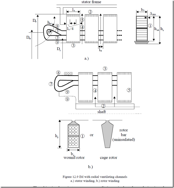
A half longitudinal cross section is shown in Figure 12.9a for the stator and in Figure 12.9b for the rotor.
The objective here is to set a more realistic equivalent thermal circuit and explicitate the various thermal resistances Rt1, … Rt9.
To do so a few assumptions are made.
• The winding end connection losses do not contribute to the stator (rotor) stack heating
• The end-connection and in-slot winding temperature, respectively, do not vary axially or radially
• The core heat center is placed ls/4 away from elementary stack radial channel
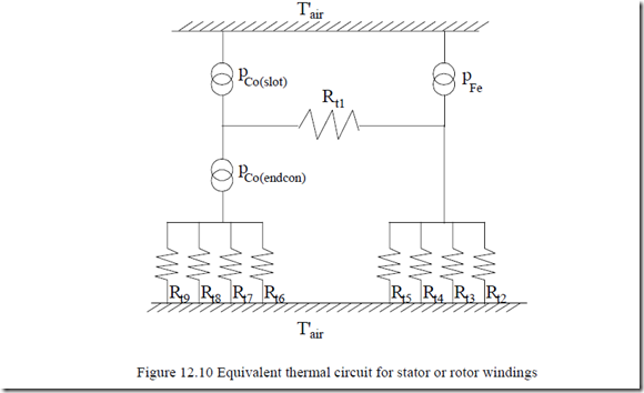
The equivalent circuit with thermal resistances is shown in Figure 12.10.
T’air – air temperature from the entrance into the machine to the winding surface.
In Figure 12.10,
PCo(slot) – winding losses for the part situated in slots
PCo(endcon) – end connection winding losses
PFe – iron losses
Rt1 – slot insulation thermal resistance from windings in slots to core
Rt2 – thermal resistance from core to air which is exterior (interior) to it – stator core to frame; rotor core to shaft
Rt3 – thermal resistance from core to airgap cooling air
Rt4 – thermal resistance from the iron core to the air in the ventilation channels Rt5 – thermal resistance from core to air in ventilation channel
Rt6 – thermal resistance towards the air inside the end connections (it is ∞ for round conductor coils)
Rt7 – thermal resistance from the frontal side of end connections to the air between neighbouring coils
Rt8 – thermal resistance from end connections to the air above them
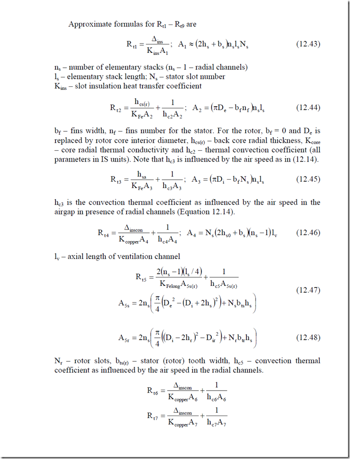
Rt9 – thermal resistance from end connections to the air below them Approximate formulas for Rt1 – Rt9 are
![]() ∆ins ; A1 ≈ (2hs + b n l Ns ) s s s (12.43)
∆ins ; A1 ≈ (2hs + b n l Ns ) s s s (12.43)
R t1 = KinsA1
ns – number of elementary stacks (ns – 1 – radial channels) ls – elementary stack length; Ns – stator slot number Kins – slot insulation heat transfer coefficient
Rt6 – Rt9 refer to winding end connection heat transfer by thermal conduction through the electrical insulation and, by convention, through the circulating air in the machine. Areas of heat transfer A6 – A9 depend heavily on the coils shape and their arrangement as end connections in the stator (or rotor).
For round wire coils with insulation between phases, the situation is even more complicated as the heat flow through the end connections toward their interior or circumferentially may be neglected (R6 = R7 = ∞).
As the air temperature inside the machine was considered uniform, the stator and rotor equivalent thermal circuits as in Figure 12.10 may be treated rather independently (pFe = 0 in the rotor, in general). In the case where there is one stack (no radial channels), the above expressions are still valid with ns = 1 and, thus, all heat transfer resistances related to radial channels are ∞ (R4 = R5 = ∞).
12.10. A DETAILED THERMAL EQUIVALENT CIRCUIT FOR TRANSIENTS
The ultimate detailed thermal equivalent circuit of the IM should account for the three dimensional character of heat flow in the machine.
Although this may be done, a two dimensional model is used. However we may break the motor axially into a few segments and “thermally” connect these segments together.
To account for thermal transients, the thermal equivalent circuit should contain thermal resistances Rti(0C/W) and capacitors Cti(J/0C) and heat sources (W) (Figure 12.11).
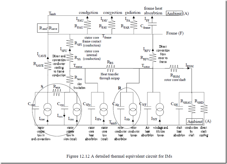
A detailed thermal equivalent circuit–in the radial plane–emerges from the more realistic thermal circuit of Figure 12.9 by dividing the heat sources into more components (Figure 12.12).
The stator conductor losses are divided into their in-slot and overhang (endconnection) components. The same thing could be done for the rotor (especially for wound rotors). Also, no heat transport through conduction from end connections to the coils section in slot is considered in Figure 12.12, as the axial heat flow is neglected.
Due to the machine pole symmetry, the model in Figure 12.12 is in fact one dimensional, that is the temperatures vary only radially. A kind of similar model is to be found in Reference [3] for PM brushless motors and in Reference 4 for induction motors.
In Reference [5], a thermal model for three-dimensional heat flow is presented.
It is possible to augment the model with heat transfer along circumferential direction and along axial dimension to obtain a rather complete thermal equivalent circuit with hundreds of nodes.
12.11. THERMAL EQUIVALENT CIRCUIT IDENTIFICATION
As shown in paragraph 12.9, the various thermal resistances Rti (or conductances Gti = 1/Rti) and thermal capacitances (Cti) may be approximately calculated through analytical formulas.
As the thermal conductivities, Ki, convection and radiation heat transfer coefficients hi are dependent on various geometrical factors, cooling system and average local temperature, and at least for thermal transients, their identification through tests would be beneficial.
Once the thermal equivalent circuit structure is settled (Figure 12.12, for example), with various temperatures as unknowns, its state-space matrix equation system is
dX = AX + BP (12.50) dt
XP==[[TP11……….TPjj……….TPnm]]tt – – power loss matrix temperature matrix (12.51)
Pj have to be known from the electromagnetic model. A and B are coefficient matrixes built with Rti, Cti.
Ideally n temperature sensors to measure T1, … Tn versus time would be needed. If it is not feasible to install so many, the model is to be simplified so that all temperatures in the model are measured.
Having experimental values of Ti(t), system (12.50) may be used to determine, by an optimization method, the parameters of the equivalent circuit. In essence, the squared error between calculated and measured (after filtering) temperatures is to be minimum over the entire time span. In Reference 6 such a method is used and the results look good.
As some of the thermal parameters may be calculated, the method can be used to identify them from the losses and then check the heat division from its center.
For example, it may be found that for low power IMs at rated speed, 65% of the rotor cage losses is evacuated through airgap, 20% to the internal frame, and 15% by shaft bearing.
Also the heat produced in the stator end connection windings for such motors is divided as: 20% to the internal frame and end shields (brackets) by convection and the rest of 80% to the stator core by conduction (axially).
Consequently, based on such results, the detailed equivalent circuit should contain a conduction resistance branch from end connections to stator core as 80% of the heat goes through it (Raxa in Figure 12.12).
As an example of an ingenious procedure to measure the Ri, Ci parameters, or the loss distribution, we notice here the case of turning off the IM and measuring the temperature decrease in location of interest versus time. From (12.18) in the steady state conditions:
ploss = R1t (T0 − Ta ) (12.52)
The temperature derivative at t = 0 (from 12.18), when the heat input is turned off, is
dTdt t 0= = − 1 (T0 − Ta ) (12.53)
R Ct t
Finally
ploss = −Ct dTdt t→0 (12.54) Measuring the temperature gradient at the moment when the motor is turned off, with Ct known, allows for the calculation of local power loss in the machine just before the machine was turned off. [7,8]


