Problem Formulation
The relations between different variables and parameters of an energy hub basically depend on the energy hub’s configuration. The configuration of a typical energy hub is depicted in Fig. 2
The calculation of objective function as well as the assumptions and technical constraints are described in this section as follows:
Energy Hub Modeling
This hub is fed by four sources of energy, namely: electric power pool (EPP), renewable energy sources (RES), gas turbines (GT), and natural gas network (NGN). It should supply two types of demand namely heat and electrical demand. It can also sell its excessive energy to the EPP. This energy hub is equipped with a CHP, electric energy storage (EES) unit. and a Furnace (F) unit.
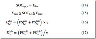
The state of charge (SOC) in energy storage device in hour t depends on SOC in hour t – 1, energy loss (EL) and the energy charge or discharge in hour t. It also depends on the scenario s. It can be described mathematically as follows:
where g is the efficiency of charge and discharge of EES unit. Echg is energy charge in EES in time t and scenario s in MWh, Edch is energy discharge in EES in time t and scenario s in MWh, SOCt;s is state of charge for EES in time t and scenario s in MWh, Eini is the initial value of state of charge at the beginning of operating horizon, Efin is the final value of state of charge at the end of operating horizon, Emax is the maximum value of state of charge, Emin is the minimum value of state of charge.
The energy storage device can be charged by using either energy hub (PShub) or by EPP (PSgrid). It also discharges to supply the hub (PSdch) or to sell its energy to
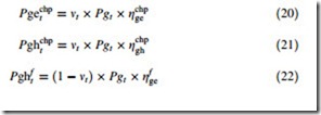
where Let;s is the electrical demand in time t and scenario s in MW, Pwt;s is the wind power generation in time t and scenario s in MW, Pet;s is the power pur- chased from EPP to supply energy hub in time t and scenario s in MW, Pgechp is the converted power from gas to electricity by CHP unit in time t in MW, Pghchp is the converted power from gas to heat by CHP unit in time t in MW, Pghf is the converted power from gas to heat by Furnace unit in time t in MW, and Lht;s is the heat demand in time t and scenario s in MW.
The internal variables of energy hub are described as follows:
where mt is the dispatch factor which specifies the share of natural gas entering the CHP or Furnace. gchp is the gas to electricity conversion efficiency of CHP unit,
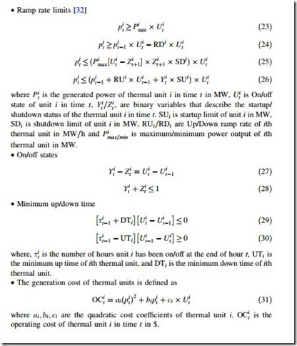
where ai; bi; ci are the quadratic cost coefficients of thermal unit i. OCi
is the operating cost of thermal unit i in time t in $.
• Total thermal units costs in time t
where, TTUCt is the total operating cost of thermal units in time t in $, STCi is the startup cost of unit i in $, and SDCi is shutdown cost of unit i in $.
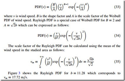
Critical Uncertainty Modeling of Wind Power Generation, Electricity Prices, and Demands The variation of wind turbine power generation is an uncertain parameter which can be probabilistically modeled using historical data records of wind speed [33, 34]. A suitable PDF for modeling the variation of wind speed, v, is found to be Rayleigh probability density function (PDF) [34], which is a special case of Weibull PDF. The mathematical expressions of Weibull PDF is as follows:
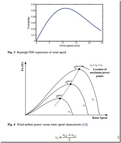
Figure 3 shows the Rayleigh PDF for b ¼ 11:28 which corresponds to vm ¼ 17:72 m=s.
For generation of wind power scenarios, a technique described in [34] is implemented in this chapter. In this techniques, the PDF of wind speed is divided into several intervals. The probability that wind speed in scenario s falls into the interval ½v1;s v2;s] i.e., v2 ½v1;s v2;s], is calculated using the following equations:
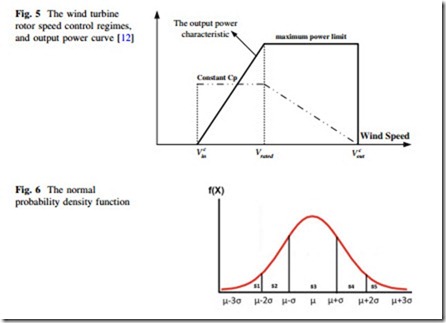
where v1;s; v2;s are the starting and ending points of the wind speed’s interval defined in scenario s (2 ½v1;s v2;s]), respectively. A typical wind turbine output power versus rotor angular speed is depicted in Fig. 4 [12]. The operating strategy of wind turbine is to adjust the rotor speed to generate power continuously close to the maximum power points which changes the power-speed characteristic. It can be accomplished by a variable speed system design and operation, which is uti- lized in the wind farms equipped by doubly fed induction generator (DFIG) [35].
In order to pick up maximum possible power from wind, the wind turbine should be operated at the peak power point at all wind speeds. By refering to
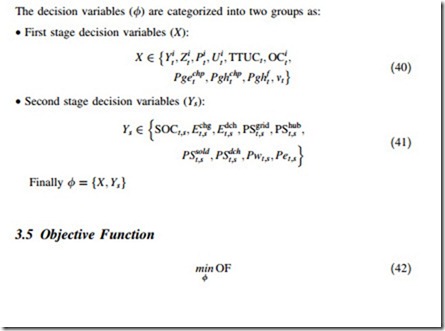
is the constant high value of tip speed ratio (TSR). Consequently, the speed and power controls in the variable speed wind power systems consist of three distinct regimes as shown in Fig. 5, where the solid curve is the output power (i.e., PwðvÞ) and the dotted curve is the rotor power coefficient (Cp) [36].
From Fig. 5, the generated power of the wind turbine is obtained using its output power characteristics and the obtained vs through (37), as follows:
Normal PDF is used for modeling the uncertainties associated with demand and electricity prices as shown in Fig. 6. As can be observed from this figure, mean (l) and variance (r) of the uncertain parameters are required for using normal PDF. According to this figure, the normal PDF is divided into 5 distinct areas. Table 1 gives the mean and the corresponding probabilities of these areas.
It is assumed that the load, price, and wind power generation states are inde- pendent, thus these states are combined to construct the whole set of states (sce- narios) as follows:
The total number of states, i.e., Ns, would be ln X kn X wn. It is obvious that for large number of scenarios (i.e., states) the computational burden of the optimization procedure drastically increased. There are some techniques to reduce the number of scenarios to decrease the computational burdens while maintaining the accuracy (see Appendix-I).
Decision Variables
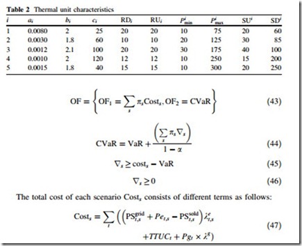
The decision variables (/) are categorized into two groups as:
• First stage decision variables (X):
The first term indicates the power flowing toward/from EPP and its associated payments. The second term is related to the operating costs of thermal units. The last term is about the gas purchase from NGN.

