The Essentials of Computer Organization and Architecture – Data Structures and the Computer

Appendix A: Data Structures and the Computer

A.1 Introduction

A civilization flourishes when people plant trees under whose shade they will never sit.

-Greek saying.

Throughout this text, we take for granted that our readers understand the basics of computer data structures. Such an understanding is not required for overall comprehension of this text, but it is helpful in grasping some of the more subtle points of computer organization and architecture. This appendix is intended as an extended glossary for readers who have yet to experience a formal introduction to data structures. It can also be used as a refresher for those who studied data structures long ago. With this goal in mind, our treatment here is necessarily brief, and it (of course!) is slanted toward hardware considerations. Readers who wish to delve further into this fascinating study are invited to read any of the books cited in the reference list at the end of this appendix. As you read through this appendix, you should be aware that all of our memory addresses in the examples are given in hexadecimal. If you haven’t already done so, you should read Chapter 2 before proceeding.

A.2 Fundamental Structures

A.2.1 Arrays

The term data structure refers to the manner in which related pieces of information are organized so that executing processes can easily access data as needed. Data structures are often independent of their implementation, as the manner of organization is logical, not necessarily physical.

The simplest of all data structures is the linear array. As you probably know from your programming experience, a linear array is a contiguous area of computer memory to which your program has assigned a name. The group of entities stored in this contiguous area must be homogeneous (they must have the same size and type) and can be addressed individually, typically using subscripting. For example, suppose you have the following Java declaration:

char[] charArray[10];

The operating system assigns a storage value to the variable charArray that represents the base address (or beginning address) of the array. Access to subsequent characters is provided through offsets from this base location. The offsets are incremented by the size of the primitive data type of the array, in this case, char. Characters in Java are 16 bits wide, so the offset for a character array would be 2 bytes per array element. For example, let’s say that the charArray structure is stored at address 80A2. The program statement:

char aChar = charArray[3];

would retrieve the 2 bytes found at memory location 80A8. Because Java indexes its arrays starting with zero, we have just stored the fourth element of the array into the character variable aChar:

 

characters offset from base address = 80A2 + 6 = 80A8.

Two-dimensional arrays are linear arrays consisting of one-dimensional arrays, so the memory offset value must take the row size into account along with the size of the primitive data type of the array. Consider for example the following Java declaration:

char[] charArray[4][10];

Here we are defining four linear arrays of linear arrays that have 10 storage locations each. However, it is much easier to think of this structure as a two-dimensional array of 4 rows and 10 columns. If the base address of charArray is still 80A2, then element charArray[1][4] would be found at address 80BE. This is because row zero of the array occupies addresses 80A2 through 80B5, row 1 starts at 80B6, and we are accessing the fifth element of the second row:

 

characters offset from base address = 80B6 + 8 = 80BE.

Array storage is a good choice when the problem that our program solves allows us to home in on a small subset of the array’s storage locations. This would be the case if we were writing a backgammon game. For example, each “point” would be a location in the “board” array. The program would inspect only those board points that are legal moves for a particular roll of the dice prior to allowing a move.

Another good application for arrays is a data collection task based on times of the day or days of the month. We might, for example, be counting the number of vehicles that pass a particular point on a highway at different times of the day. If someone later asks for the average traffic flow between 9:00 and 9:59 am, all we need to do is average the tenth element of each 24-hour day’s array for the period over which we have collected the data. (Midnight to 1:00 am is the zeroth element.)

A.2.2 Queues and Linked Lists

Arrays are not very helpful when we are processing items in response to requests for service. Requests for service are usually processed according to the time that the request was made. In other words, first come, first served.

Consider a Web server that handles Hypertext Transfer Protocol (HTTP) requests from users connected through the Internet. The sequence of incoming requests may resemble the one shown in Table A.1.

Table A.1: HTTP Requests for a Web Server

Conceivably, we could place each of these requests into an array and then search the array for the lowest timestamp value when we are ready to service the next request. This implementation would be hopelessly inefficient, however, because each element of the array would need to be interrogated every time. Furthermore, we would risk running out of room in the array if we experience a day with an unusually heavy amount of traffic. For these reasons, a queue is the appropriate data structure for first-come, first-served applications. The queue data structure requires that elements be removed in the same order in which they are entered. Waiting lines at banks and supermarkets are good examples of queues.

There are different ways to implement queues, but all queue implementations have four components: a memory variable that points to the first item in the queue (the head of the queue), a memory variable that points to the end of the queue (its tail), memory locations in which to store the queue items, and a set of operations specific to the queue data structure. The pointer to the head of the queue indicates which item is to be serviced next. The tail pointer is useful for adding items to the end of the queue. When the head pointer is null (zero), the queue is empty. The operations on queues typically include adding an entry to the end of the list (enqueue), deleting an entry from the beginning of the list (dequeue), and checking to see whether the queue is empty.

One popular way of implementing a queue is to use a linked list. In a linked list, each item in the queue contains a pointer to the next item in the queue. As items are dequeued, the head pointer can use the information found in the node that was just deleted to locate the next node. So, in our web server example above, after Item 1 is serviced (and removed from the queue), the head-of-queue pointer is set to point to Item 2.

In our example from Table A.1, let’s say that the head of the queue is at address 7049, which contains the first HTTP request, www.spiffywebsite.com/sitemap.html . The head-of-queue pointer is set to the value 7049. At memory address 7049, we will have the entry:

07:22:03, 10.122.224.5, www.spiffywebsite.com/sitemap.html, 70E6

where 70E6 is the address of the following item:

07:22:04, 10.167.14.190, www.spiffywebsite.com/shoppingcart.html, 712A.

The entire contents of the queue are shown in Table A.2.

Table A.2: An HTTP Request Queue Implemented in Memory

The pointer to the head of the queue is set to 7049 and the tail pointer is set to 81B3. If another user request arrives, the system finds a spot for it in memory and updates the last queue item (to point to the new entry), as well as the tail pointer. You should notice that when this kind of pointer structure is used, unlike arrays, there is no requirement that the data elements be contiguous in memory. This is what enables the structure to grow as needed. Moreover, there is no requirement that the addresses be ascending, as we have shown. The queue elements can be located anywhere in memory. The pointers maintain the order of the queue.

The queue architecture that we have described can be modified to create a fixed-size queue (often called a circular queue), or a priority queue, where certain types of entries will jump ahead of the others. Even with these added wrinkles, queues are easy data structures to implement.

A.2.3 Stacks

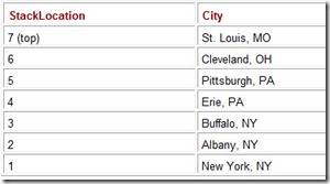
Queues are sometimes called FIFO (first-in, first-out) lists, for obvious reasons. Some applications call for the opposite ordering, or last-in, first-out (LIFO). Stacks are appropriate data structures for LIFO ordering. They get their name from their similarity to how cafeterias provide plates to their customers. Cafeteria service personnel add hot, wet, clean plates to the top of a spring-loaded tube, pushing the cold, dry plates further down the tube. The next customer takes a plate from the top of the stack. This sequence is shown in Figure A.1. Figure A.1a shows a stack of plates. The plate numbered 1 was the first one placed on the stack. Plate number 7 was the last. Plate number 7 is the first plate removed, as shown in Figure A.1b. When the next plate arrives, plate number 8, it will go on top of the stack as shown in Figure A.1c. The act of adding an item to a stack is called pushing. To remove an item is to pop it. To interrogate the top item in a stack, without removing it, is to peek at it.

A stack is a useful data structure when you are working your way through a series of nested subroutine calls in a program. If you push the current address on the top of the stack before you branch to the next address, you know that you can return along the same route as you arrived. All you do is pop each address as you need it. As an example from everyday life, say we visit a series of cities in this order:

1. New York, NY

2. Albany, NY

3. Buffalo, NY

4. Erie, PA

5. Pittsburgh, PA

6. Cleveland, OH

7. St. Louis, MO

8. Chicago, IL

From Chicago, how do we get back to New York? A human being would simply pull out a map (and find a more direct route), or would just “know” to find Interstate 80 and head east. Computers certainly aren’t as smart as we are. So the easiest thing for a computer to do is to retrace its original route. A stack (like the one shown in Table A.3) is exactly the right data structure for the job. All that the computer needs to do is push the current location on the top of the stack as the route is traversed. The return route is easily found by popping the previous city from the top of the stack.

Table A.3: A Stack of Visited Cities

It is possible to implement stacks in a variety of ways. The most popular software implementations are done via linear arrays and linked lists. System stacks (the hardware versions) are implemented using a fixed memory allocation, which is a block of memory set aside for the exclusive use of the stack. Two memory variables are required to manage the stack. One variable points to the top of the stack (the last item placed onto the stack), while a second variable keeps a count of the number of items in the stack. The maximum stack size (or the highest allowable memory address) is stored as a constant. When an item is pushed onto the stack, the stack pointer (the memory address for the top of the stack) is incremented by the size of the data type that is stored in the stack.

Consider an example where we want to store the last three letters of the alphabet and retrieve them in reverse order. The Java (Unicode) coding for these characters in hexadecimal is:

X = 0058, Y = 0059, Z = 005A.

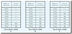
Memory addresses 808A through 80CA are reserved for the stack. A constant, MAXSTACK, is set to 20 (hex). Because the stack is initially empty, the stack pointer is set to a null value, and the stack counter is at zero. Table A.4 shows a trace of the stack and its management variables as the three Unicode characters are stored.

Table A.4: Adding the Letters X, Y, and Z to a Stack. (The dashes represent irrelevant memory values.) a. X (0058) Is Added and the Stack Pointer Is Incremented by the Size of the Data Element (2 Bytes) b. Y (0059) Is Added and the Stack Pointer Is Incremented by 2 Again c. Z (005A) Is Added

To retrieve the data, three pops take place. With each pop, the stack pointer is decremented by two. Of course with each addition and retrieval, the status of the stack must be checked. We have to be sure that we don’t add an item to a stack that is full or try to remove an item from a stack that is empty. Stacks are widely used in computer system firmware and software.

A.3 Trees

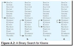
Queues, stacks, and arrays are useful for processing lists of things where the locations of the items within the list (relative to each other) do not change no matter how many items are in the list. Certainly, this is not the nature of many of the data collections that we use in our daily lives. Consider a program that would manage an address book. One useful way of sequencing this data is to keep the list in order by last name. A binary search could quickly locate any name in the list, successively limiting the search to half of the list. A binary search is shown seeking the name Kleene within the list of famous mathematicians in Figure A.2. We begin by determining the middle of the list (Hilbert) and comparing this value to our key. If they are equal, we have found the desired item. If the key (Kleene) is larger than the item in the middle of the list, we look in the bottom half of the list, as shown in Figure A.2b. (This effectively reduces our search space by half.) Now, we determine the new middle (Markov) of the bottom half of the list. If our key (Kleene) is smaller than this new middle, we throw out the bottom half of this list and keep the top half, as in Figure A.2c. If our key has still not been found, we divide the list in half again. In this way, we successively divide the list in half until we find our key (or determine that it is not in the list). This example was contrived to show a worst-case situation. It took 4 operations to locate a key in a list of 16 items. If it happened that we were looking for Hilbert, we’d have found him on the first try. No matter how large the list is, any name could be located in time proportionate to the base 2 logarithm of the number of items in the list.

Clearly, a binary search requires that the data be sequenced by its key values. So what happens when we want to add a name to our address book? We must put it in its proper place so that we can reliably use the binary search. If the book is stored in a linear array, then we can quite easily figure out where the new element belongs, say at position k. But to insert this item, we must make room for it in the array. This means that we must first move all of the items at locations k through n (the last item in the book) to locations k + 1 through n + 1. If the address book is large, this shifting process would probably be slower than we would like. Furthermore, if the array can hold only n items, we are in big trouble. A new array will have to be defined and then loaded from the old one, consuming even more time.

A linked list implementation won’t work very well, either, because the midpoint of the list is hard to find. The only way to search a linked list is to follow the chain of list items until you find the spot where the new item should be. If you have a long list, linear searches are operationally infeasible-they won’t happen fast enough to make anyone happy.

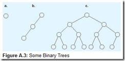
So a good data structure for keeping ordered, maintainable lists is one that allows us to find things quickly yet add and delete items without excessive overhead. There are several data structures that fit the bill. The simplest of these is the binary tree. Like linked lists, binary trees keep track of adjacent data items through the use of pointers to memory locations. And, like linked lists, they can grow arbitrarily large. But this growth is done in such a way that it’s easy to retrieve any key from the tree. Binary trees are called binary because in their graphical representation each node (or vertex) has at most two descendant (child) nodes. (Trees with more than two descendant nodes are called n-ary trees.) Some example binary trees are shown in Figure A.3. Don’t let it bother you that these graphics look like upside-down trees-they are trees in the mathematical sense. Each node is connected to the graph (meaning that every node is reachable from the first node), and the graph contains no cycles (meaning that we can’t end up going in circles as we’re looking for things).

The topmost node of a tree is its root. The root is the only part of a tree that has to be kept track of independently. All other nodes are referenced through the root using two memory pointer values stored in each node. Each pointer indicates where the node’s left child or right child node can be found. The leaves of a tree, nodes at the very bottom of the structure, have null values for their child nodes. The distance, the number of levels, from the leaves to the root of a tree is called its height. Nodes that are not leaves are called internal nodes of the tree. Internal nodes have at least one subtree (even if it’s a leaf).

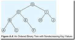
In addition to pointers, the nodes of a binary tree contain data (or data key values) around which a tree is structured. Binary trees are often organized so that all key values smaller than the key value at a particular node are stored in its left subtree and all key values greater than or equal to the key value are stored in its right subtree. Figure A.4 shows an example of this idea.

The binary tree shown in Figure A.4 is also a balanced binary tree. Formally, when a binary tree is balanced, the depth of the left and right subtree of every node differ by at most 1. What is significant about this is that any data item referenced by the tree can be located in time proportionate to the base 2 logarithm of the number of nodes in the tree. So a tree containing 65,535 data keys requires at most 15 memory operations to find any particular element (or to determine that it’s not there). Unlike sorted lists kept in linear arrays (that give the same running time for a search) it is much easier to maintain the set of key values in binary trees. To insert an element, all we do is rearrange a few memory pointers, rather than restructure the entire list. The running time for both inserting and deleting a node from a balanced binary tree is also proportionate to the base 2 logarithm of the number of items in the tree. Thus, this data structure is much better than an array or simple linked list for maintaining a group of sorted data elements.

Although our graphics make it easy to conceptualize the logical structure of a tree, it is good to keep in mind that computer memory is linear, so our picture is only an abstraction. In Table A.5, we have provided a map of 64 bytes of memory that store the tree in Figure A.4. For convenience of reading, we show them in a tabular format. For example, the hex address of the byte located in the column with label 5 (which we will refer to as Column 5) of the row with label 1 (Row 1) is 15. Row 0, Column 0 refers to address 0. The node keys are coded in hexadecimal ASCII, as shown in the table above the memory map.

Table A.5: The Memory Map for the Binary Tree in Figure A.4.

In our memory map, the root of the tree is located at addresses 36 through 38 (Row 3, Columns 6-8). Its key value is at address 37. The left subtree (child) of the root is found at address 25, and the right subtree at address 3B. If we look at address 3B, we find the key, I, with its left child at address 14, and its right child at address 21. At address 21, we find the leaf node, J, having zeroes for both of its child pointers.

Binary trees are useful in many applications such as compilers and assemblers. (See Chapter 8). However, when it comes to storing and retrieving key values from very large data sets, several data structures are superior to binary trees. As an example, consider the task of designing an online telephone book for New York City, which has a population of just over 8 million people. Assuming that there are approximately 8 million telephone numbers to put in our book, we would end up with a binary tree having at least 23 levels. Furthermore, over half of the nodes would be at the leaves, meaning that most of the time, we would have to read 22 pointers before finding the desired number.

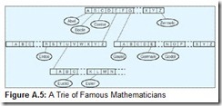
Although a binary tree design is not totally dreadful for this application, we can improve upon it. One better way involves an n-ary tree structure called a trie (pronounced “try”). Instead of storing an entire key value in each node, tries use fragments of the keys. The key value is assembled as a search proceeds down the trie. Internal nodes contain a sufficient number of pointers to direct a search to the desired key or to the next level of the trie. Tries are particularly suitable for data having variable-length keys, such as our telephone book example. Shorter keys are near the top, whereas longer keys are at the bottom of the data structure.

In Figure A.5, we have depicted a trie containing the names of famous mathematicians. The diagram implies that every internal node contains 26 letters. The nature of our data suggests that there are more efficient trie structures than the one shown. (We observe that it is hard to find a famous mathematician whose name begins with ZQX.) In fact, designing an internal node structure is the hardest part of trie construction. Depending on the key values, more than one character can be used as an index. For example, suppose that instead of containing each letter of the alphabet as a single unit, we could use groups of letters. By changing the multiplicity of the keys in the root node of the trie in Figure A.5, the trie can be made flatter by one level. This modification is shown in Figure A.6. A consequence of flattening the trie is that searching can be done faster, if such flattening is done carefully. In Figure A.6, we chose to roll up only two keys, ER and EU, to eliminate one level. If we had doubled up every key, the root would contain 676 keys (AA through ZZ), making the data structure unnecessarily large and unwieldy with respect to the amount of data that it stores.

In practice, structures for storage and retrieval of large amounts of data are designed with more consideration to the medium upon which they will be stored than to the nature of the data itself. Often, index nodes are contrived so that some integral number of internal nodes at one level of the tree is accessible through one read operation of the disk drive upon which the index is stored. One such data structure is a B+ tree, which is used in large database systems.

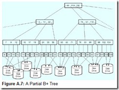
A B+ tree is a hierarchical structure consisting of pointers to index structures or actual data records. As records are added and deleted from the database, leaves in the B+ tree are updated. Additional branches (internal nodes) are spawned when updates to existing leaves are not possible. The internal nodes of a B+ tree are collectively referred to as its index part, whereas the leaf nodes are called the sequence part, because they will always be in sequential order. A schematic of a portion of a B+ tree is shown in Figure A.7.

The numbers shown in the diagram are record key values. Along with each key value in the leaf node of a B+ tree, the database management system (see Chapter 8) maintains a pointer to the location of the physical record. This pointer value is used by the operating system to retrieve the record from the disk. So the physical record can be located virtually anywhere, but the sequence part of the data structure always stays in order. Traversal of the B+ tree assures us that any record can be located quickly based on its key value.

To locate a key value using the B+ tree shown in Figure A.7, all we need to do is compare the desired value with the values stored in the internal nodes. When a key value is less than the value of a key in an internal node, the tree is traversed to the left. Accordingly, retrieving a value greater than or equal to an internal node’s key value requires that we traverse the tree to the right. When an internal node has reached its capacity, and we need to add a record to the database, additional levels are added to the hierarchy. Record deletion, however, does not cause an immediate flattening of the tree, just a movement of pointers. B+ tree hierarchies are flattened during a process called database reorganization (or reorg). Reorgs can be exceedingly time-consuming in large databases, so they are usually performed only when absolutely necessary.

The best database indexing methods take into account the underlying storage architecture of the systems upon which they run. In particular, for best system performance, disk reads must be kept to a minimum. (See Chapter 10.) Unless a substantial part of a data file’s index is cached in memory, record accesses require at least two read operations: one to read the index and another to retrieve the record. For B+ tree indices on highly active files, the first few levels of the tree are read from cache memory rather than from disk. Thus, disk reads are required only when retrieving lower index tree levels and the data record itself.

A.4 Network Graphs

By definition, tree structures contain no cycles. This makes trees useful for data storage and retrieval, a simple task in terms of computational complexity. Harder problems require more complex structures. Consider, for example, the routing problem that we presented in Section A.2, where we need to find a return path from Chicago to New York. We never said anything about finding the shortest path, only that it was easiest to simply retrace our steps. Finding the shortest path, or an optimal path, requires a different kind of data structure, one that allows cycles.

An n-ary tree can be changed into a more general network graph by allowing leaf nodes to point to each other. But now we have to allow for the fact that it is possible for any node to point to the remaining n – 1 nodes in the graph. If we simply extend the binary tree data structure to allow for a network data structure, each node would need n – 1 pointers. We can do better.

If the network in question is static, that is, it neither gains nor loses nodes through the execution of our algorithm, it can be represented using an adjacency matrix. An adjacency matrix is a two-dimensional array with a row and column for each node. Consider the graph shown in Figure A.8a. It has six interconnected nodes. The connections (edges) between the nodes of the graph are indicated by a 1 in the adjacency matrix, where the column of one node and the row of the other intersect. The completed adjacency matrix is shown in Figure A.8b.

Let’s return to our example of finding an optimal route between two cities. We represent the map as a graph with weighted edges. The weights on the edges correspond to the distance, or “cost” of going from one city to another. Instead of entering 1s into the adjacency matrix, these traveling costs are entered where a route between two cities exists.

It is also possible to represent a connected graph as a linked adjacency list. The implementation of an adjacency list structure usually involves keeping the nodes of the graph in a linear array that points to a list of nodes to which it is adjacent. The nice part about this arrangement is that we can easily locate any node in the graph, and the cost of moving between one node and another can be kept in the list elements coming off of the array. Figure A.9 shows a weighted graph along with its adjacency list data structure.

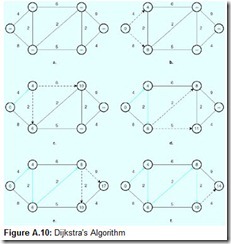
General graphs, such as the ones we have been describing, are widely used for solving communications routing problems. One of the most important of these algorithms is Dijkstra’s algorithm, which works on the idea that the least-cost route through the graph consists of the collection of all of the shortest connecting links between all of the nodes. The algorithm starts by inspecting all paths adjacent to the starting node of the graph. It updates each node with the cost of getting there from the starting node. It then inspects each path to adjacent nodes, updating each with the cost of getting to the node. If the node already contains a cost, it is selected as the next destination only if the cost of traveling to that node is smaller than the value already recorded in that node. This process is illustrated in Figure A.10.

In Figure A.10a, the value to reach all nodes is set to infinity. Paths from the first node to its adjacent nodes are inspected, and each node is updated with the cost of getting to that node (Figure A.10b). Paths from the node of lesser cost to its neighbors are inspected, updating those nodes with the cost to reach them, if that cost is less than the value that was previously stored in each node. This is what happens to the node at the lower left-h and side of the graph in Figure A.10c. The process repeats until the shortest path is discovered, as shown in Figure A.10f.

One of the tricky parts of Dijkstra’s algorithm is that a number of data structures are involved. Not only does the graph itself have to be provided for, but the paths to each node have to be recorded somehow so that they can be retrieved when needed. We leave as an exercise the matter of representing the required data structures and the construction of pseudocode for Dijkstra’s algorithm that operates on those data structures.

Summary

This appendix has described a number of important data structures commonly employed by computer systems. Stacks and queues are most important at the lowest levels of the system, because the simplicity of these data structures matches the simplicity of the operations that take place at those levels. At the system software level, compilers and database systems rely heavily on tree structures for fast information storage and retrieval. The most complex data structures are found at the high-level language layer. It is possible for these structures to consist of more than one subsidiary data structure, as in our illustration of a network graph that uses both an array and a linked list to fully describe the graph.

Exercises

1. Give at least one example of applications where each of the following data structures would be most suitable:

   1. Arrays

   2. Queues

   3. Linked lists

   4. Stacks

   5. Trees

2. As stated in the text, a priority queue is a queue in which certain items are allowed to jump to the head of the line if they meet certain conditions. Devise a data structure and a suitable algorithm to implement a priority queue.

3. Suppose you didn’t want to maintain a set of sorted data elements as a tree, but chose a linked list implementation instead, despite its obvious inefficiencies. The list is ordered by key values in ascending order, that is, the lowest key value is at the head of the list. To locate a data element, you search the list linearly until you find a key value that is greater than the key value of the item’s key. If the purpose of this search is to insert another item into the list, how would you achieve this insertion? In other words, give a pseudocode algorithm that lists each step. You can make this algorithm somewhat more efficient by slightly changing the data structure of the list.

4. The memory map shown below describes a binary tree. Draw the tree.

   

5. Hints and Answer The memory map shown below describes a binary tree. Draw the tree.

   

6. The memory map shown below describes a binary tree. The leaves contain the keys H (48), I (49), J (4A), K (4B), L (4C), M (4D), N (4E), and O (4F). Draw the tree.

   

7. Devise a formula for the maximum number of nodes that can be placed in a binary tree with n levels.

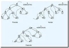
8. A graph traversal is the act of interrogating (or visiting) every node in the graph. Traversals are useful when nodes are added to a tree in a certain order (perhaps random) and retrieved in some other given order. Three frequently used traversals, preorder, inorder, and postorder, are shown in the diagram below, with diagram a illustrating a preorder traversal, b an inorder traversal, and c a postorder traversal.

   

   1. Rearrange the tree above so that a preorder traversal will print the node key values in alphabetical order. Change only the key values in the nodes. Do the same for an inorder traversal.

   2. Perform the other two traversals on both of the trees redrawn in Part a.

9. Most books concerning algorithms and data structures present traversal algorithms as recursive procedures. (Recursive procedures are subroutines or functions that call themselves.) However, the computer achieves this recursion using iteration! The algorithm below uses a stack to perform an iterative preorder traversal of a tree. (Refer to the previous question.) As each node is traversed, its key value is printed as in the diagram above.

   ALGORITHM Preorder
      TreeNode : node
      Boolean : done
      Stack: stack
      Node ¬ root
      Done ¬ FALSE
      WHILE NOT done
         WHILE node NOT NULL
            PRINT node
            PUSH node onto stack
            node ¬ left child node pointer of node
         ENDWHILE
         IF stack is empty
            done ¬ TRUE
         ELSE
            node ¬ POP node from stack
            node ¬ right child node pointer of node
         ENDIF
      ENDWHILE
   END Preorder

   1. Modify the algorithm so that it will perform an inorder traversal.

   2. Modify the algorithm so that it will perform a postorder traversal. (Hint: As you leave a node to follow its left subtree, update a value in the node to indicate that the node has been visited.)

10. Regarding the trie root node shown in Figure A.6, what complications arise if we discover a famous mathematician whose name is Ethel? How can we prevent this problem?

11. Using Dijkstra’s algorithm, find a shorter route from New York to Chicago using the mileages given in the adjacency matrix below. The value “infinity” (¥) indicates no direct connection between two given cities.

    

12. Suggest a way in which an adjacency matrix could be stored so that it will occupy less main memory space.

13. Design an algorithm, with suitable data structures, that implements Dijkstra’s algorithm.

14. Which of the data structures discussed in this appendix would be the best for creating a dictionary that would be used by a spelling checker within a word processor?