The application of 3D computational fluid dynamics
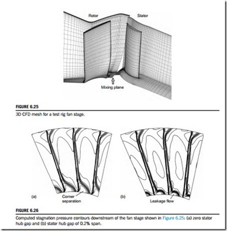
Three-dimensional computational fluid dynamics (CFD) started to be developed in the 1970s and early 1980s. The first methods were inviscid and ran on very coarse meshes of only a few thousand points per blade passage. These methods were generally based on the Euler blade-to-blade approach, described in Chapter 3, extended to three dimensions. Viscous 3D CFD became possible in the 1980s due to the advances made in computing. Much larger meshes, of the order of 100,000 points, are required to resolve viscous flow features like boundary layers close to the blade surfaces. More powerful computers enabled the full equations of motion, with viscous terms, to be solved for such meshes. 3D CFD is now routinely applied to the analysis and design of turbomachinery, and solutions with mesh sizes of around 1 million points can be computed in less than a few hours on a modern workstation. Figure 6.25 shows an example of a viscous CFD mesh for a low-speed fan with 1 million points in the rotor mesh and 0.64 million in the stator. Note how the mesh points are clustered together close to the blade and endwall surfaces.
Most methods applied to turbomachinery use time-marching algorithms, where the solution iterates towards convergence. These methods require a turbulence model to “close” the equations of motion and this introduces an element of uncertainty into the accuracy of a prediction, even when an extremely fine mesh is used. In general, flow features that are not particularly sensitive to turbulence are still well predicted, whereas some viscous and 3D flow features are difficult to reproduce accurately (Denton and Dawes, 1999). A modern 3D CFD method, if applied carefully, should reliably predict the blade surface pressure distribution, the primary flow field, transonic effects, any effects of lean and sweep, and any leakage flows. However, secondary flows and surface boundary layers, which depend on the parameters of the inlet boundary layers and on the turbulence model, may be inaccurate. For example, 3D CFD has difficulty predicting the extent of corner separations in compressors and often some empirical calibration is required. Figure 6.26 shows the predicted flow downstream of the fan stage illustrated in Figure 6.25. Results are shown for the stator with no hub gap, Figure 6.26(a), and for a small stator hub gap of 0.2% span, Figure 6.26(b). The computed results in Figure 6.26(a) can be compared directly with the measured results given earlier in Figure 6.21. Although the predicted flow field includes comparable features, there are significant
differences: the predicted corner separation is larger, the predicted wake has higher loss, and the flow structure close to the casing is different. Figure 6.26(b) shows that a small amount of leakage flow is potentially beneficial in reducing the size of the corner separation.
A comprehensive presentation of the limitations of CFD is given in Denton (2010) and phenomena that are shown to be particularly difficult to predict include boundary layer transition, viscous shear and mixing, trailing edge flows, and compressor stall. Despite these issues, CFD remains an
invaluable tool for turbomachinery design and analysis, provided it is applied carefully with a full understanding of its capabilities.
Single-passage steady computations
Many single-passage computations are still performed for turbomachinery design and analysis, and before the introduction of multirow computations, CFD could only be applied to single blade rows in isolation. For such computations, it is essential to ensure that the boundary conditions applied are accurate. These can be extracted from a through-flow computation of the whole machine, and this is the normal approach for design work, or alternatively, experimental measurements of the inlet and exit flow field are applied as boundary conditions.
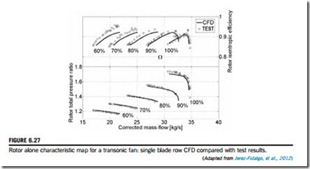
Figure 6.27 shows an example of predicted performance results from single-passage steady CFD of a transonic fan rotor, from Jerez-Fidalgo, Hall, and Colin (2012). The agreement between CFD and experimental data shown here is better than average. There is a close match in the shape of all the characteristic curves and the absolute levels of pressure ratio and choking mass flow are accurately reproduced. However, the stall point is not predicted accurately, and should not be expected to be, since stall is inherently unsteady and involves the full-annulus flow field. Also, at part speeds, the predicted efficiency values are noticeably lower than the measured values.
Multiple blade row steady computations
In general, the flow around a rotor blade is steady in the relative frame and the flow around a stator blade is steady in the stationary frame. However, wakes and pressure perturbations generated by a rotor will be perceived by an adjacent downstream stator as unsteady fluctuations.
Unsteady interactions between the components are, therefore, always present, but rather than compute the complete time-accurate unsteady flow field, which is computationally very expensive, there are some techniques that enable the time-averaged unsteady flow to be predicted for multistage machines using just steady computations.
The most straightforward and common approach is to simply average the flow field in the circumferential direction at the exit of each blade row. The flow conditions will then be steady in both frames of reference and they can then be exchanged as a boundary condition to the down- stream blade row. The averaging process is equivalent to mixing the flow and, therefore, the interfaces between the rotating and stationary blade rows are called mixing planes (as shown in Figure 6.25). The problem with mixing planes is that the mixing, or averaging, introduces extra loss at the interfaces and, in general, this will be different from the loss that would have occurred if the circumferentially nonuniform flow had been allowed to interact and mix unsteadily in the downstream blade passage.
Another approach developed by Adamczyk (1985) was to use deterministic stresses that describe all the effects of unsteadiness linked to the machine shaft rotation rate. This method allows steady computations to be used, but extra terms are included in the momentum equations that capture the gradual mixing of the flow from upstream blade rows. This has been shown to give improved results relative to mixing planes, but it requires a more complex computational method, and either a model of the deterministic stresses must be provided or larger, overlapping grids are required to calculate how these stresses vary downstream of each blade row.
Unsteady computations
Unsteady 3D computations are currently too expensive and time-consuming to perform routinely for turbomachinery design. However, they are necessary for problems where unsteady phenomena are important and they are widely used in research and development. For example, unsteady CFD can be applied to investigating blade row interactions, compressor stall and surge, noise generation, nonuniform installation effects, and unsteady secondary flow features. These fields are active areas of research and well beyond the scope of this book, but it is worth stating that advanced unsteady CFD methods combined with huge computational resources are enabling continuous improvements in our understanding of complex turbomachinery aerodynamic problems.
Current and future application of CFD to turbomachinery
Over the last 20 years, turbomachinery design has becoming increasingly more dependent on 3D CFD, and this trend is set to continue. Simple methods of determining performance with empirical input, such as described in this book, are still needed for the mean radius design and for through-flow calculations. It is often emphasized by experienced designers that, if the one-dimensional preliminary design is incorrect, e.g., the blade diffusion factors and stage loading, then no amount of CFD will produce a good design! However, CFD does provide the ability to exploit the 3D nature of the flow to suppress deleterious features, such as corner stall in compressors or strong secondary flows in turbines. It is also a quick means to provide better understanding of the flow field for a given design.
As indicated by Horlock and Denton (2003), loss predictions from CFD are still not accurate and interpretation of the computations requires considerable skill and experience. Denton (2010)
shows there are still a large number of limitations in CFD that users need to be aware of and these are areas requiring further research and development.
The outlook for CFD is that its capabilities will continue to develop and that it will be used more routinely to tackle more complex turbomachinery design and analysis problems. This trend has been apparent for some time and, at the turn of the century, Adamczyk (2000) outlined the shift towards multistage and unsteady flow computations with more detailed geometrical features and larger computational meshes. The speed and availability of cluster computing has enabled larger computations to be done in shorter and shorter timescales. Figure 6.28 shows the computational domain for the calculation of a high-speed fan stage operating within a test facility with a nonuniform inlet flow field (Jerez-Fidalgo et al., 2012). The mesh contains over 40 million points and the CFD used is fully viscous and unsteady. Computations of this type, in just the last few years, have gone from taking months to run, to just weeks and now, in some cases, days. In the future, computations that were previously barely feasible for research will become routine and possible within design timescales. The growing challenge will be to process the large quantities of data produced by such computations and to interpret the results correctly. Also, with greater computational capabilities, there are inevitably going to be fewer rig tests, which tend to be very expensive, and, there- fore, fewer opportunities for experimental validation. The future CFD user should maintain a healthy amount of skepticism in their results!


