DC Servo Motors for Very High Performance Requirements
For high performance applications, the inductance of the motor and the flexibility of the transmission mechanism must be considered. A schematic diagram of such system is shown in Fig. 4.9. It is assumed that a gearbox with input and output speed ratio of N, is attached to the motor. In practice, often a lead screw is attached to the gearbox to transfer the rotational displacement to linear displacement. The stiffness of the lead screw is assumed to be Ks. The stiffness is determined from the design parameters of the transmission mechanism. The stiffness changes as the length of the lead screw changes. The worst condition when the stiffness is minimum must be considered for design of the controller.
For position control, a position feedback must be used. It is better to derive the system governing differential equation in open loop and to study various control strategies later. The voltage equation of the DC motor may be written as
s is the Laplace operator and Cm is the voltage constant. The last term in Eq. (4.9) is the internal velocity feedback, which helps to increase damping of the system. It should be noted that θm is the angular position of the rotor and it is different from the angular position of the load because the transmission mechanism is assumed to be flexible. The output torque is proportional to the current and the equation of motion becomes
The term on the left hand side of the above equation is the torque developed by the rotor. The parameters Jm, C, Tr are the rotor inertia, the mechanical damping referred to the motor, and the external torque referred to the rotor respectively. The torque transferred to the transmission mechanism is
N is the gearbox speed ratio and Ts, θo, Ks is the torque applied to the motor, the output poison, and the stiffness of the transmission mechanism. The equation of the motion for the load may be written as
The parameters Jl, Cl, Tl are the load inertia, the damping ratio of the transmission mechanism and the external torque applied to the motor.
The above equations are all the differential equations that describe the dynamic behavior of the DC servo motor in general form. There is now various methods to study the dynamics of the system and to design a proper controller to achieve the required performance. One method is to use the principle of superposition and to find the transfer function of the system in which the output position is related to the two input variables of voltage and external torque. The proportional, proportional plus integrator, and lead-lag network may be studied to find an acceptable compro- mise between the required accuracy and speed of response. For this purpose, the Nyquist diagram, Bode diagram, or the root locus may be used. It should be noted that the characteristic equation of the system will be of order of five and if Integral or lead-lag control strategy is used the order of the system will increase. With classi- cal control strategy it is not possible to move all the roots to required position on the s-plane. The reader is encouraged to do the manipulation by substituting numerical values by obtaining a catalogue from the manufacturer. With numerical values the reader should be able to design various classical control strategies. It should be noted that a velocity feedback and position feedback directly from the motor usually are provided by manufacturers of DC servo motors.
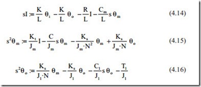
In this section, state variable feedback control strategy is studied. There is no need to find the overall transfer function. By carefully manipulating the governing differential equations, they can be converted to a form that it is possible to define state variables that are measurable directly by high performance transducers. By eliminating TsTr from Eqs. (4.9)–(4.13) the governing equations can be converted to three sets of differential equations; that is,
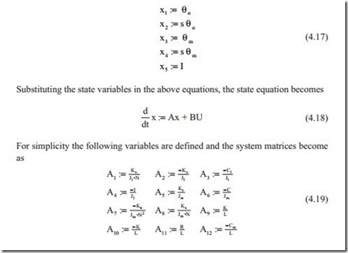
Equations (4.14)–(4.16) are now in a form that it is possible to define state variables. The current motor position and velocity, output position, and velocity are all the state variables that are directly measurable with high performance transducers. The following state variables are defined as
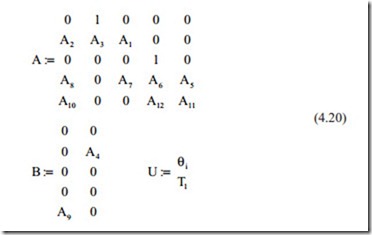
Note that the usual brackets for the matrices are not shown.
The reader is warned to see that the subscript of J and T in Eq. (4.17) is the lower case L. It can be seen that there are five state equations. The subscript of C in Eq. (4.17) is again lower case L showing the effect of viscous friction in the load side and C in Eq. (4.17) is the viscous friction at the motor side. At the design stage, the two coefficients of viscous damping may not be known. For simplicity, these two coefficients may be set to zero to consider the worst conditions. When the system is designed the friction coefficients can be measured and the analysis may be improved a better performance design specifications.
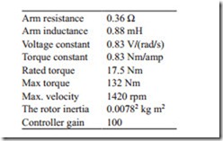
Equation (4.17) now is the form that was described in Chap. 4. It is desirable first to study the open loop system equation. For this, it is required that numerical values are substituted in the system equation and the eigenvalues of the system matrix A gives the roots of the characteristic equation. From the position of the eigenvalues on the s-plane a state variable feedback control strategy can be studied. The reader is encouraged to derive the system equation by doing the manipulations to ensure that the system equation is correct. A DC servo motor with the following specifica- tions is considered:
Arm resistance 0.36 Ω Arm inductance 0.88 mH
Voltage constant 0.83 V/(rad/s) Torque constant 0.83 Nm/amp Rated torque 17.5 Nm
Max torque 132 Nm
Max. velocity 1420 rpm
![]() The rotor inertia 0.00782 kg m2 Controller gain 100
The rotor inertia 0.00782 kg m2 Controller gain 100
It can be seen that the maximum torque, which is available for a short period of time, is much larger than the rated torque, which can be used continuously. It can be proved by the energy consideration that torque and voltage constants are equal for
100 % efficient motors. The motor in consideration is separately excited. The trans- mission mechanism can be idealized by a shaft with stiffness of 1000 Nm/rad. This is an example for the sake of numerical analysis. For real application, the stiffness must be calculated from the design configuration of the system.
It is assumed that a gearbox is attached to the motor with input/output speed ra- tio of N = 10. For most poison control servos, a gearbox must be used to reduce the speed to an acceptable level. The DC servo motors are available at various output torque and speed configurations depending on the design of motor. Various motors must be tried to find the most suitable one. For the purpose of analysis the power unit is considered an ideal amplifier that converts low-level signal to high voltage and current output. The properties of various power units will be studied at the end of this chapter. Selecting a motor can be started by matching the load inertia to the motor inertia. The rule of thumb is that they should be equal or less than the rotor inertia. In this calculation, the effect of gearbox which reduces the effect of load inertia by a factor of 1/N2 must be taken into account. In this example, it is assumed that the load inertia is 0.078 kg m2. The MathCad software is used to study the dy- namic behavior of the system as follows:
The eigenvalues (the roots of the characteristic equation) are calculated with MathCad software by substituting the numerical parameters in the matrix equations and calculating the eigenvalues of the system matrix as follows.
It can be seen that three are five eigenvalues with two complex conjugate and one real eigenvalue. The first two complex conjugates show the structural oscillation one due rotor and load inertia and one the link between the magnetic field and rotor. The real parts of the second complex roots are very small showing that there will be seviour oscillation. The real root is very small showing slow response because it is very small. If the position feedback was not used a zero root would have appeared showing that there will be a free motion. Without the position feedback the equa- tions can be written in terms of motor speed. The real parts of one of complex roots are positive showing that with control gain as 100 the system is unstable. Suppose it is desired to keep the gain as 100 and it is required by designing state variables feedback to move all roots to a desired location on the s-plane.
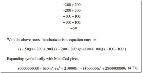
It should also be noted that the real root is very small and it should be increased to a position further away from the imaginary axis. Suppose that it is required to move all roots to the following position on the s-plane. This means that all complex roots must have a damping ratio of 0.7 and the real root is moved to − 50 positions giving a time constant of 0.02 s.
With the above roots, the characteristic equation must be
 State variable feedback control strategy can now be implemented in two ways. One method as described in Chap. 4 is to measure all state variables and feed them as
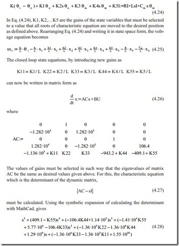
positive to the input variable θi. The second method is to inject the state variables immediately after the proportional control. Because already a position feedback is used the second method will be used. A positive feedback is considered and the gains might become positive or negative depending on the state matrix. The voltage equation then becomes
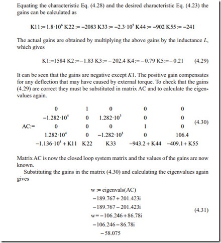
The actual gains are obtained by multiplying the above gains by the inductance L, which gives
It can be seen that the gains are negative except K1. The positive gain compensates for any deflection that may have caused by external torque. To check that the gains (4.29) are correct they must be substituted in matrix AC and to calculate the eigen- values again.
Matrix AC is now the closed loop system matrix and the values of the gains are now known.
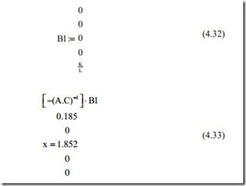
Substituting the gains in the matrix (4.30) and calculating the eigenvalues again gives
It can be seen from the eigenvalues (4.31) that indeed the eigenvalues have been moved to the required value. There are slight differences, which are due to the rounding off error.
It can be seen that the roots of the characteristic equation all have a damping ratio of greater than 0.7 because the real part of the roots have moved to the left of − 45° line on the complex plane. The real root has moved to the required position on the complex plane. There has been a small change in the required values of the eigenvalues due to a rounding off error in the calculation. This indicates that the eigenvalues are not very sensitive to the values of gains. This is useful for practical applications where the exact gains might be achievable. The reader is encouraged to change each gain by approximately 10 % to observe how sensitive the eigenvalues are when the gain is changed.
In this section, the matching of the coefficients of desired and actual character- istic is used to calculate the gains. There are other methods, which are beyond the scope of this book. For servo motors applications, the author finds that the above method is very useful. The method can also be used for simpler applications.
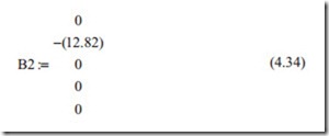
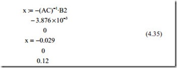
After calculating the gains, it is useful to investigate the steady state values of the state variables to study the accuracy of the closed loop system. The calculations for unit step input of θi and external torque of zero is as follows:
The above analysis shows that the two output positions move to a position different from the required unit one. This is no problem as input can be calibrated in terms of output position. It is also noted that the motor rotates ten times the output position. This was expected. The current also becomes zero at steady state since the motor has moved to the correct position, there is no need for current.
It is also important to study the effect of external torque by using the principle of superposition. For this the input is set to zero and for unit input of external torque the method of calculation is as in Eqs. (4.32) and (4.33). First, the input vector of the external torque is calculated.
The same procedure for calculation of unit step input is used. The results become
It can be seen that the errors are very small and when the maximum rated torque of approximately 10 N m is used the error just becomes ten times greater than the value given above. It should be noted that units of all rotation is in radian. It should also be noted that there is a current of 0.12 A passes through the motor to try to correct the position.
For greater accuracy, the roots must be moved further away from the real axis of the s-plane. For zero steady state error, an integrator must be added in the forward path of the system. This increases the order of the system from 5–6 and the system becomes more complicated. The reader is encouraged to study this as final year or master project. In this case it may not be possible to measure all state variables. The use of full order or reduced order observer must be studied.
The purpose above was to show that for servo motor writing the governed differential equations in above form all state variables could be measured for feedback. All roots also can be moved to required position on the s-plane.


