Design Example
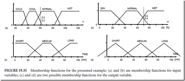
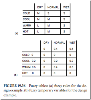
Consider the design of a simple fuzzy controller for a sprinkler system. The sprinkling time is a function of humidity and temperature. Four membership functions are used for the temperature, three for humidity, and three for the sprinkle time, as shown in Fig. 19.35. Using intuition, the fuzzy table can be developed, as shown in Fig. 19.36(a).
Assume a temperature of 60◦F and 70% humidity. Using the membership functions for temperature and humidity the following fuzzy variables can be obtained for the temperature: (0, 0.2, 0.5, 0), and for
the humidity: (0, 0.4, 0.6). Using the min operator, the fuzzy table can be now filled with temporary fuzzy variables, as shown in Fig. 19.36(b). Note that only four fields have nonzero values. Using fuzzy rules, as shown in Fig. 19.36(a), the max operator can be applied in order to obtain fuzzy output variables: short → o1 = max{0, 0, 0.2, 0.5, 0} = 0.5, medium → o2 = max{0, 0, 0.2, 0.4, 0} = 0.4, long → o3 = max{0, 0} = 0. Using Eq. (19.47) and Fig. 19.35(c) a sprinkle time of 28 min is determined. When the simplified approach is used with Eq. (19.46) and Fig. 19.35(d), then sprinkle time is 27 min.
Genetic Algorithms
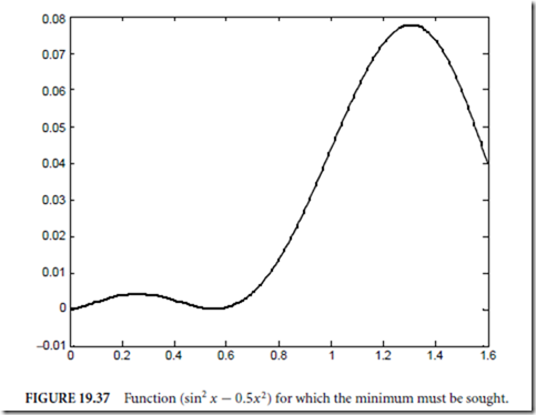
The success of the artificial neural networks encouraged researchers to search for other patterns in nature to follow. The power of genetics through evolution was able to create such sophisticated machines as the human being. Genetic algorithms follow the evolution process in nature to find better solutions to some complicated problems. The foundations of genetic algorithms are given by Holland (1975) and Goldberg (1989). After initialization, the steps selection, reproduction with a crossover, and mutation are repeated for each generation. During this procedure, certain strings of symbols, known as chromosomes, evaluate toward a better solution. The genetic algorithm method begins with coding and an initialization. All significant steps of the genetic algorithm will be explained using a simple example of finding a maximum
of the function (sin2 x − 0.5x)2 (Fig. 19.37) with the range of x from 0 to 1.6. Note that in this range, the function has a global maximum at x = 1.309, and a local maximum at x = 0.262.
Coding and Initialization
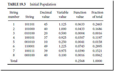
At first, the variable x has to be represented as a string of symbols. With longer strings, the process usually converges faster, so the fewer the symbols for one string field that are used, the better. Although this string may be the sequence of any symbols, the binary symbols 0 and 1 are usually used. In our example, six bit binary numbers are used for coding, having a decimal value of 40x. The process starts with a random generation of the initial population given in Table 19.3.
Selection and Reproduction
Selection of the best members of the population is an important step in the genetic algorithm. Many different approaches can be used to rank individuals. In this example the ranking function is given. Highest rank has member number 6, and lowest rank has member number 3. Members with higher rank should have higher chances to reproduce. The probability of reproduction for each member can be obtained as a fraction of the sum of all objective function values. This fraction is shown in the last column of Table 19.3. Note that to use this approach, our objective function should always be positive. If it is not, the proper normalization should be introduced at first.
Reproduction
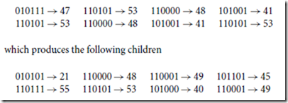
The numbers in the last column of Table 19.3 show the probabilities of reproduction. Therefore, most likely members number 3 and 8 will not be reproduced, and members 1 and 6 may have two or more copies. Using a random reproduction process, the following population, arranged in pairs, could be generated
If the size of the population from one generation to another is the same, two parents should generate two children. By combining two strings, two other strings should be generated. The simplest way to do this is to split in half each of the parent strings and exchange substrings between parents. For example, from parent strings 010100 and 100111, the following child strings will be generated 010111 and 100100. This process is known as the crossover. The resultant children are
In general, the string need not be split in half. It is usually enough if only selected bits are exchanged between parents. It is only important that bit positions are not changed.
Mutation
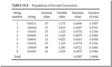
In the evolutionary process, reproduction is enhanced with mutation. In addition to the properties inherited from parents, offspring acquire some new random properties. This process is known as mutation. In most cases mutation generates low-ranked children, which are eliminated in the reproduction process. Sometimes, however, the mutation may introduce a better individual with a new property. This prevents the process of reproduction from degeneration. In genetic algorithms, mutation usually plays a secondary role. For very high-levels of mutation, the process is similar to random pattern generation, and such a searching algorithm is very inefficient. The mutation rate is usually assumed to be at a level well below 1%. In this example, mutation is equivalent to the random bit change of a given pattern. In this simple case, with short strings and a small population, and with a typical mutation rate of 0.1%, the patterns remain practically unchanged by the mutation process. The second generation for this example is shown in Table 19.4.
Note that two identical highest ranking members of the second generation are very close to the solution x = 1.309. The randomly chosen parents for the third generation are
The best result in the third population is the same as in the second one. By careful inspection of all strings from the second or third generation, it may be concluded that using crossover, where strings are always split in half, the best solution 110100 →52 will never be reached, regardless of how many generations are created. This is because none of the population in the second generation has a substring ending with 100.
For such crossover, a better result can be only obtained due to the mutation process, which may require many generations. Better results in the future generation also can be obtained when strings are split in random places. Another possible solution is that only randomly chosen bits are exchanged between parents.
The genetic algorithm almost always leads to a good solution, but sometimes many generations are required. This solution is usually close to global maximum, but not the best. In the case of a smooth function the gradinet methods are converging much faster and to a better solution. GA are much slower, but more robust.
Defining Terms
Backpropagation: Training technique for multilayer neural networks.
Bipolar neuron: Neuron with output signal between −1 and +1.
Feedforward network: Network without feedback. Perceptron: Network with hard threshold neurons. Recurrent network: Network with feedback.
Supervised learning: Learning procedure when desired outputs are known.
Unipolar neuron: Neuron with output signal between 0 and +1.
Unsupervised learning: Learning procedure when desired outputs are unknown.
References
Fahlman, S.E. 1988. Faster-learning variations on backpropagation: an empirical study. Proceedings of the Connectionist Models Summer School, eds. Touretzky, D. Hinton, G., and Sejnowski, T. Morgan Kaufmann, San Mateo, CA.
Fahlman, S.E. and Lebiere, C. 1990. The cascade correlation learning architecture. Adv. Ner. Inf. Proc. Syst., 2, D.S. Touretzky, ed. pp. 524–532. Morgan, Kaufmann, Los Altos, CA.
Goldberg, D.E. 1989. Genetic Algorithm in Search, Optimization and Machine Learning. Addison-Wesley, Reading, MA.
Grossberg, S. 1969. Embedding fields: a theory of learning with physiological implications. Journal of Mathematical Psychology 6:209–239.
Hebb, D.O. 1949. The Organization of Behivior, a Neuropsychological Theory. John Wiley, New York. Hecht-Nielsen, R. 1987. Counterpropagation networks. Appl. Opt. 26(23):4979–4984.
Hecht-Nielsen, R. 1988. Applications of counterpropagation networks. Neural Networks 1:131–139. Holland, J.H. 1975. Adaptation in Natural and Artificial Systems. University. of Michigan Press, Ann Arbor,MI.
Hopfield, J.J. 1982. Neural networks and physical systems with emergent collective computation abilities.
Proceedings of the National Academy of Science 79:2554–2558.
Hopfield, J.J. 1984. Neurons with graded response have collective computational properties like those of two-state neurons. Proceedings of the National Academy of Science 81:3088–3092.
Kohonen, T. 1988. The neural phonetic typerater. IEEE Computer 27(3):11–22.
Kohonen, T. 1990. The self-organized map. Proc. IEEE 78(9):1464–1480.
Kosko, B. 1987. Adaptive bidirectional associative memories. App. Opt. 26:4947–4959.
Kosko, B. 1988. Bidirectional associative memories. IEEE Trans. Sys. Man, Cyb. 18:49–60.
McCulloch, W.S. and Pitts, W.H. 1943. A logical calculus of the ideas imminent in nervous activity. Bull.
Math. Biophy. 5:115–133.
Minsky, M. and Papert, S. 1969. Perceptrons. MIT Press, Cambridge, MA.
Nilsson, N.J. 1965. Learning Machines: Foundations of Trainable Pattern Classifiers. McGraw-Hill, New York.
Nguyen, D. and Widrow, B. 1990. Improving the learning speed of 2-layer neural networks, by choosing
initial values of the adaptive weights. Proceedings of the International Joint Conference on Neural Networks (San Diego), CA, June.
Pao, Y.H. 1989. Adaptive Pattern Recognition and Neural Networks. Addison-Wesley, Reading, MA.
Rosenblatt, F. 1958. The perceptron: a probabilistic model for information storage and organization in the brain. Psych. Rev. 65:386–408.
Rumelhart, D.E., Hinton, G.E., and Williams, R.J. 1986. Learning internal representation by error propagation. Parallel Distributed Processing. Vol. 1, pp. 318–362. MIT Press, Cambrige, MA.
Sejnowski, T.J. and Rosenberg, C.R. 1987. Parallel networks that learn to pronounce English text. Complex Systems 1:145–168.
Specht, D.F. 1990. Probalistic neural networks. Neural Networks 3:109–118.
Specht, D.F. 1992. General regression neural network. IEEE Trans. Neural Networks 2:568–576.
Wasserman, P.D. 1989. Neural Computing Theory and Practice. Van Nostrand Reinhold, New York.
Werbos, P. 1974. Beyond regression: new tools for prediction and analysis in behavioral sciences. Ph.D.
diss., Harvard Universtiy.
Widrow, B. and Hoff, M.E., 1960. Adaptive switching circuits. 1960 IRE Western Electric Show and
Convention Record, Part 4 (Aug. 23):96–104.
Widrow, B. 1962. Generalization and information storage in networks of adaline Neurons. In Self- organizing Systems, Jovitz, M.C., Jacobi, G.T. and Goldstein, G. eds. pp. 435–461. Sparten Books, Washington, D.C.
Wilamowski, M. and Torvik, L. 1993. Modification of gradient computation in the backpropagation algorithm. ANNIE’93—Artificial Neural Networks in Engineering. November 14–17, 1993, St. Louis, Missou.; also in Dagli, C.H. ed. 1993. Intelligent Engineering Systems Through Artificial Neural Networks Vol. 3, pp. 175–180. ASME Press, New York.
Zadeh, L.A. 1965. Fuzzy sets. Information and Control 8:338–353.
Zurada, J. M. 1992. Introduction to Artificial Neural Systems. West Publishing Company, St. Paul. MN.
