Risk Management
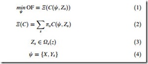
Suppose an objective function Cðw; ZÞ, in which, W is the decision variable vector and Z are the input uncertain parameters. If the probability density functions of the uncertain parameters are known then these parameters can be described using scenario-based approach and treated with two-stage optimization techniques. The scenario-based approach divides the uncertain continuous universe of discourse for parameter Z into jXsj scenarios with specific probabilityps. The next step is the proper treatment of optimization procedure. The two-stage optimization technique states that the decision variable vector W consists of two types of variables. the first type are called ‘‘here and now’’ or ‘‘first stage’’ variables and are denoted by X. These variables remain the same for all possible scenarios. The second type of the variables are called ‘‘wait and see’’ or ‘‘second stage’’ variables and are denoted by Ys. These variables are determined specifically for each scenario s.
where Nð:Þ is expected value operator. ps is the probability of scenario s. The main problem with this approach is ignorance of the risk. The term ‘‘risk’’ can be interpreted in many ways depending on the context it is being used. Formally, it is defined as a situation involving exposure to an undesired event which is mainly due to the existence of uncertainties involved in decision-making procedure. This event may be an unpleasant technical, economical, or environmental situation. Each risk management strategy involves answering the following questions [16]:
• What can happen?
• How to quantify the impacts/risk measures?
• What are the consequences?
• What are the preventive/remedial actions?
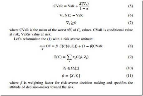
The methods of risk modeling can be divided into different categories [17], namely; fuzzy methods [18], scenario-based methods [19–21], information gap decision theory (IGDT)-based methods [22, 23], and robust optimization [24]. In context of the scenario-based models, there are various methods for quantifying the risk impacts such as variance [25], shortfall probability [26], stochastic dominance [27], value at risk VaR [28], and CVaR [29]. In this chapter, the CVaR method is used as a risk measure. The CVaR is defined as the expected value of losses exceeding the VaR. While the VaR gives the frequency of extreme events, CVaR considers not only the frequency but also the severity of losses in case of undesired events [30]. For example, although the expected value of cost function Cðw; ZsÞ is minimized but the decision-maker may still face with severe outcomes in some scenarios with low probability. Comparing with VaR, CVaR is a more conservative index, because it measures the average loss exceeding the VaR value for a given confidence level [31]. CVaR is defined as follows:
where b is weighting factor for risk averse decision making and specifies the attitude of decision-maker toward the risk.


