Eigenvalues, Eigenvectors, and Characteristic Equation
The state variable equations, which are in the form of n first order differential equation, can also be solved like ordinary differential equations. Because state equations are written in matrix form some extra terms must be taken into account. Like for ordinary differential equation two solutions of transient and steady state can be assumed. To find the transient solution, the input vector are set to zero and state equations become
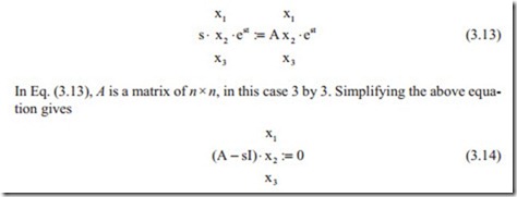
In Eq. (3.12), it is clear that the values of x1, x2, x3 give the amplitude of each state variable and should be distinguished from the state variables. The second term in Eq. (3.12) determines weather the system is unstable, stable, overdamped, or underdamped. Substituting from Eq. (3.12) in Eq. (3.11) and after some algebraic manipulation gives
I is unit matrix with diagonal terms 1 and off diagonal terms zero. It is clear that Eq. (3.14) is an eigenvalue problem. The eigenvalues are the roots of characteristic equation. This will be shown for the above example. The matrix ( A − sI) is known as dynamic matrix. The eigenvector associated with each eigenvalue has some mean- ing in vibrations as it gives the mode shape but in control has only meaning when the output has to be calculated. With numerical integration method there is no need to go into details of other methods.
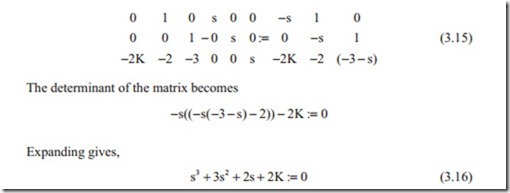
Equation (3.14) has a nontrivial solution if the determinant of the dynamic matrix is zero. The first example in the above sections will be considered, this gives
It can be seen that the determinant of the dynamic matrix is the same as that of char- acteristic equation. There are computer programs such as MathCAD which gives the eigenvalues of the dynamic matrix and there is no need to calculate the characteristic equation. The MathCAD may be used to obtain the characteristic equation in symbolic form and polyroots (v) statement may be used to calculate the roots for various parameters.
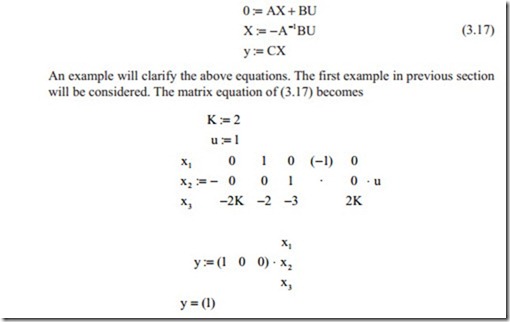
When the stability is assured, the steady state value of the output variables can be obtained by setting all derivatives to zero and solving n linear equation as follows:
It can be seen that for k = 2 and input u = 1 the output is also 1, which means that the steady state error is zero. For input other than step, it is better to solve the dif- ferential equation. One method is solving the differential equation numerically. In this case by definition,
In the above equation, T is the time interval and t is the time. The process can be started from t = 0 and the calculation can be repeated to obtain the solution over the required time interval. In the above equation, X can be considered as the state variable vector. Substituting for d X from Eq. (3.6) into above equation giving the solution for state variables,
In Eq. (3.18), A is the system matrix and B is the input matrix. The time interval T must be sufficiently small to avoid numerical instability. Then, sufficiently large time span must be selected to give the response. The time interval and the time span can be selected with respect to eigenvalues. The input variable may be a single vari- able or could be a vector U if more than one input variable exist.
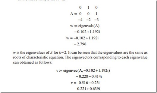
The eigenvalues of matrix A can be calculated making use of various software such as MathCad. In this method, the eigenvalues can be calculated as
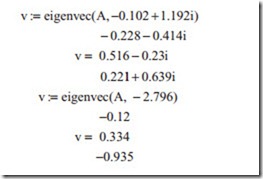
As it was discussed earlier, for each eigenvalue there is a corresponding eigenvec- tor. This process can be repeated for all eigenvalues as follows:
For complex conjugates eigenvalues, there are also two conjugate eigenvectors. For real root, there is a real eigenvector. The eigenvectors will be used to assess the controllability and observability of the control system.

