Important Features of Root Locus
Usually the transfer function of elements of a control system is in form of first or second order lag form and the closed loop system is in the form of several cascaded of these transfer functions. This can be used to sketch the root locus manually from the open loop transfer functions. There are important features on the Root Locus that the loci can be sketched manually and they are useful to know. It can be used for simple system and it is very complicated for complex systems.
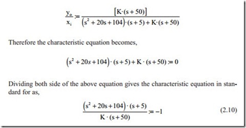
Without loss of generality consider the simple system shown in Fig. 2.5.
Where xi is the input variable and ( yo) is the output variable to be controlled. The second order term in the denominator could be as a mass-spring-damper transfer equation. The other term in the numerator and in the denominator may represent a lead lag compensation network. The K is the parameter of interest that should be adjusted to obtain a stable and fast responding system.
The angle Law states that the angle of left side of Eq. 2.10, which is a complex number, should be ± 180° measured from the real axis counter clockwise.
The magnitude law states that the magnitude of the left side of Eq. (2.10) should be − 1.
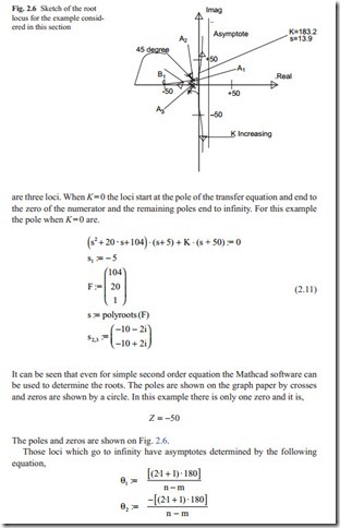
These two laws and some feature of the loci help us to draw the root locus manually. The order of the denominator is n = 3 and the order the numerator is m = 1 for the open loop transfer function. From the characteristic equation is clear that there
1 is any integer number. For real systems the complex roots appears in conjugate so for this complex conjugate there is one positive and one negative asymptote. Select- ing one for the integer l = 1 the angle of asymptotes becomes,
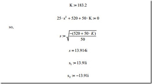
The value of k must be as such that the first column must be all positive for the sys- tem to remain stable. Doing this the value of K where the loci crosses the imaginary axis can be found. The first column of third row indicates that the value of K must be less than 183.2. The first column of forth row is more complicated because there is the K to power of 2 and the denominator has also the coefficient K. It is clear that for k = 183.2 the first column fourth row for the above K is positive. To find the in- tersections points on the imaginary axis the auxiliary equation is formed as,
These points are shown on the imaginary axes by crosses. The reader is encourage to do the Routh–Hurwitz algebra themselves to show the data presented here is cor- rect. For design purpose the value of K must be selected to have a damping ratio 0.7. This damping ratio is achievable by drawing a 45° line from the origin and its intersection with the loci gives a damping ratio of 0.7. The following procedures remain as before only the magnitude changes. This is shown by point A on the loci. Then the value of gain is obtained by magnitude law as,
By remembering these important points the root locus can be sketched manually on a graph paper as shown in Fig. 2.6. This is just an approximate of the root locus and for complicated system, the procedures becomes complex. It is useful to know these points and when the root locus is plotted using a software like Mathcad these point can be identified on the plot. Even the above procedures are only valid when the open loop and feedback loop transfer function appears of in a simple cascaded form.
For design purposes poles and zeros can be added to pull the loci to the desired position and in this example a lead-lag network were added to improve the speed of response with sufficient damping in the system.
Now the Mathcad mathematical software is used to plot the root locus from calculating the roots of characteristic equation.
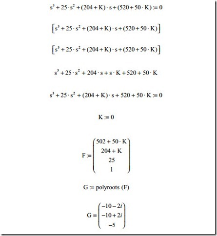
The characteristic equation of the closed loop can be calculated easily as was calculated above as is given below for reference purposes.
The characteristic equation has been expanded symbolically and with such power software there is no need do the calculation manually.
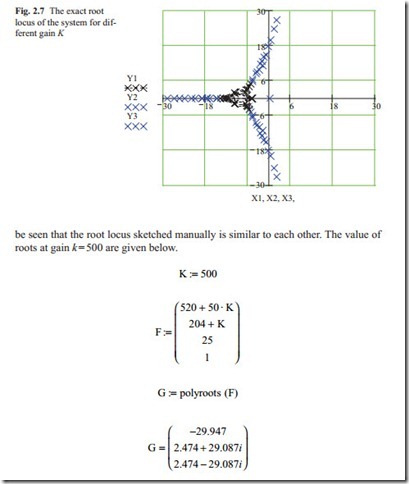
The process is repeated up to the point, when the root locus of interest is plotted. Figure 2.7 shows the root locus plotted from the gain K = 0 to the gain K = 500. It can
The root locus is plotted by calculating the roots at different values of gain. For each gain the roots were put in an array and then the results were plotted on the graph. Each root is shown by a cross. Because of many gains the roots were put in three arrays and then plotted. It can be seen that the two root locus are similar. In fact there is no need to plot the root locus because trying few gains it is possible to find the correct roots location to have fast response with sufficient damping in the system. It is also possible to add zeros and poles to improve the system response.
