Geographic Diversity
The most important influencer of the uncertainty and variability of aggregate wind power is the geographic diversity of the system. A system’s geographic diversity is a reference to the general level of dependence between the wind power from its constituent wind plants. Dependence is often quantified using a correlation coefficient, with lower correlation generally resulting in decreased uncertainty and variability. The goal of this section is to formulate the mathematic basis for this phenomenon, discuss factors influencing correlation and dependency, as well as to comment on practical considerations.
Theoretical Basis
Aggregate wind power can mathematically be represented as
where P~agg is the normalized aggregate wind power, N is the number of wind plants considered, and Ci and Pi are the capacity and real power delivered by the ith wind plant.
Hereafter, subscripts are used to associate a variable with a specific wind plant, so that xn pertains to the nth wind plant. We start with the idealized assumption that the wind speed at each wind plant ~v1; .. .; ~vN are independent random variables. Consequently, P~1; .. .; P~N will also be independent random variables, and are therefore uncorrelated.
As a result of the assumption of independence, the probability distribution of the aggregate power output is found through convolution and change-of-variables:
where lagg and ragg are the mean and standard deviation of fPagg P~agg . The transformation of the probability density function to a Gaussian distribution according to the Central Limit Theorem has important implications to the uncertainty of aggregate wind power.
Uncertainty and Variability Reduction
The normalized aggregate wind power’s statistical variance will decrease as more wind plants are added to the system according to
where r2 is the variance of the normalized power output of the ith wind plant. The decrease in variance causes the Gaussian distribution to contract, which can be interpreted as a decrease in the uncertainty of the wind power.
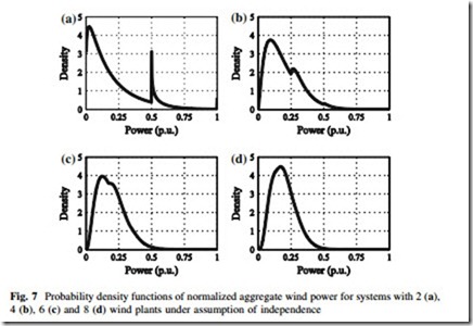
The evolution of fPagg P~agg to a Gaussian distribution can be noticeable even for small values of N. This is illustrated in Fig. 7 where fPagg P~agg for N = 2, 4, 6, and 8 are plotted using numerical convolution based on the pdf in Fig. 5a and assuming independence in power output. Note how the distribution contracts as more wind plants are aggregated, resulting in decreased standard deviation and decreased probability of extremely high or low power output. In other words, the uncertainty decreases.
The effects of geographic diversity also apply to the moment-to-moment variation in aggregate wind power: under the assumption of independence, as more wind plants are aggregated the moment-to-moment variation approaches a Gaussian distribution with decreasing variance.
The preceding derivation showed the mathematical mechanism by which geographic diversity reduces uncertainty and variability in aggregate wind power. Its foundation is the assumption that the wind speed (and power) at all N wind plants are independent, and hence not correlated, but how realistic and restrictive is this assumption? It is intuitive that a pair of wind plants in close proximity will experience similar wind conditions. However, if they are separated by several hundred kilometres, the same claim becomes unreasonable. In other words, wind power tends to exhibit high spatial dependency of its correlation. It is these features that ultimately determine the geographic diversity of a system.
Correlation of Instantaneous Wind Power
The dependency of two random variables can be quantified by correlation coefficients. The correlation coefficient does not fully capture the underlying dependency structure between the variables as the joint distribution would, but nonetheless it is useful in quantifying the dependency. Among the most used correlation coefficients are Pearson’s q and Kendall’s s. Pearson’s q measures linear correlation, whereas Kendall’s s measures rank correlation [35]. There is no compelling reason to believe that wind power would be linearly correlated, and it has been argued that Kendall’s s is a more suitable metric for wind speed or power [36]. Nonetheless, many studies to date have focused strictly on Pearson’s q. Whichever metric is used, it is widely recognized that there exists a strong relationship between separation distance and correlation coefficient [10–16].
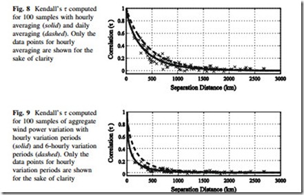
Empirical studies have shown that the relationship between separation distance and correlation coefficient can be modeled as
where r is the so-called decay constant, s is the stretching coefficient, and d is the distance between wind plants in kilometers [7, 16]. Figure 8 shows the computed Kendall’s s for various randomly sampled wind plant pairings obtained from the NREL Eastern Wind Integration Data Set [37]. Similar traces have been reported for Pearson’s q [7, 14]. The solid trace is for hourly averaged data; the dashed trace is for daily-averaged data. The decay and stretching coefficients for the hourly averaged data are 0.0037 and 0.92, respectively; and 0.0096 and 0.81 for the daily averaged data, respectively. In general, longer averaging periods result in larger correlation coefficients. Zero correlation in wind power among wind plant pairs does occur but is rare, and when it does occur it is usually at separation distances greater than 1,000 km.
Correlation of Wind Power Variation
Geographic diversity tends to have more pronounced effect on the moment-to- moment variation of wind power than on instantaneous wind power. Figure 9 shows the rank correlation coefficient for variation periods of 1 h (solid) and 6 h (dashed) for the same 100 wind plant pairs that were considered in the previous section. As before, an equation of the form of (19) suitably fits the data. The decay and stretching coefficients are 0.108 and 0.532 for the hourly variation, and 0.029 and 0.692 for the 6-hourly variation, respectively. From Fig. 9, and in general, longer variation periods tend to have higher correlation than short ones.
When compared to instantaneous power, the correlation coefficients of wind power variations are smaller and decay faster with distance. Near-zero correlation is exhibited at closer distances, around 750 km. The reduction of variation (smoothing effect), therefore, is noticeable in many systems.
Other Factors Influencing Correlation
Correlation of wind power is not solely dependent on separation distance. Other variables influencing correlation of wind power are:
• Terrain. Wind plants located close to each other but in different terrain may experience different wind regimes, which may decrease correlation.
• Averaging and variation period. Shorter periods tend to exhibit less correlation. Compare, for example, the solid and dashed lines in Figs. 8 and 9.
• Direction of the separation. For example, many North America wind plants with East–West separation have greater correlation than those with North–South separation [38].
• Number of wind turbines. Correlation between aggregate wind power in systems tends to be higher than the correlation between wind plants of individual wind turbines [16]. High frequency fluctuations tend to be uncorrelated and are filtered by dispersed wind turbines.
It is also notable that the correlation coefficient itself may exhibit erratic variation. Wind plant pairs may exhibit high correlation one day, and low correlation the next [15, 18].
Wind Power Dependency Structures
The correlation coefficient, while useful in quantifying dependence, does not provide sufficient information to construct the pdf of aggregate wind power from a pair of wind plants. Rather, information on the dependency structure of the wind power contained in the pair’s joint distribution is needed.
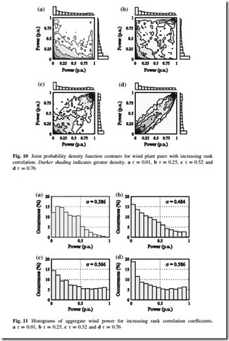
The dependency structure of wind power is best explained visually and by considering the bi-variate case. Figure 10 shows typical, yet specific, contour plots of joint probability density functions for four different wind plant pairs, each with different rank correlation coefficients. The darker shading indicates greater density. The marginal histograms are shown on the top and right side of each plot.
Inspecting Fig. 10 shows how rank correlation tends to influence the joint distribution of wind power. At the lowest levels of correlation (Fig. 10a), mutually high power output is rare. Mutually low power output does occur, but that is an artifact of the marginal distributions having increased density at low power output.
At correlation levels in Fig. 10b—around 0.25—a concentration of higher density appears in the area of mutually high power output, but the density at mutually lower power remains. As correlation increases (Fig. 10c, d), the density begins to align along the diagonal, with areas of increased density at the extremes.
The normalized power output from each wind plant pair can be summed to examine the aggregate wind power in each of the four cases. The resulting histograms of aggregate power are shown in Fig. 11. Note that the power has been re- normalized by dividing the aggregate power by two, using a simplifying assumption that the capacities of each wind plant are identical.
As can be expected from its near-zero correlation, Fig. 11a resembles a system with higher geographic diversity. The standard deviation is lower than the others, and there is decreased probability of extreme power output. As correlation increases in Fig. 11b–d, so does the standard deviation and propensity for extreme power output. In Fig. 11d, the histogram appears similar to that of an individual wind plant, which is a signature of low geographic diversity.
Figure 11 also illustrates that the wind plants in a system do not need be uncorrelated to realize the benefits of geographic diversity. Rather, uncertainty and variability are decreased even if the wind plants exhibit higher correlation— although not as noticeably as if the wind plants are uncorrelated.
Multivariate Models and Simulation
In the special case that aggregate and individual wind power need to be modeled or simulated, a multivariate model is required. For example, a Monte Carlo simulation can be performed by sampling from the joint distribution of the power from the wind plants. However, a proper joint distribution model must be identified.
Returning to Fig. 10, we see that the joint distributions do not obviously con- form to any common parametric functions, and are certainly not Gaussian. One reason for this is that the marginal distributions add complexity to the overall structure. It is possible to decouple the influence of the marginal distributions from the joint by transforming the data from the wind power domain to the rank/uniform domain by way of the cdf of the individual wind plants. The result is uniform marginal distributions, with a joint distribution that is more amenable to parametric modeling. The resulting dependency structure can be modeled using copulas [39]. Though beyond the scope of this chapter, other works have shown that Gumbel and Gaussian copulas are appropriate for multi-variate wind power dependency modeling [40, 41]. The selection of a specific copula depends on the number of wind plants and the desired rank correlation.
One method of Monte Carlo simulation of wind power using copulas is: (1) identify the separation distances of the wind plants to be modeled; (2) using (19), compute the corresponding rank correlation matrix; (3) select an appropriate multivariate copula to model the dependency structure, using the correlation coefficient to determine the copula’s parameters; (4) randomly draw the desired number of samples from the copula in the rank/uniform domain; (5) transform the samples to the wind power domain using the inverse cdf of (7). See [40, 41] for additional implementation details.
Practical Considerations
Geographic diversity can theoretically reduce uncertainty and variability of aggregate wind power. However, in many systems, the perceived benefits of geographic diversity have failed to materialize. There are four main reasons for this [16]:
1. In many electricity markets, the system-wide benefits of reduced uncertainty and variability do not directly translate into gains for individual wind plants— they do not have compelling economic reasons to seek geographic diversity.
2. Wind plants tend to have greater capacities, resulting in high concentrations of wind turbines.
3. There is limited access to suitable transmission limits the number of geo- graphically diverse regions that can be interconnected.
4. There is only so much geographic diversity that can be had. In a given region,
as wind plants are added, the benefits of geographic diversity saturate. Additionally, large-scale forces such as insolation similarly influence very wide areas (e.g., the continental United States).
In this section we have shown that geographic diversity, particularly in the separation distance between wind plants, reduces dependency and correlation. This in turn leads to a transformation of the probability density function of instantaneous and moment-to-moment variations in aggregate wind power toward a Gaussian distribution, with decreased standard deviation, and hence less uncertainty and variability. However, geographic diversity can and should not be viewed as a panacea for eliminating variability and uncertainty. Wind plants exhibit statistically significant correlation at large separation distances, and there are several practical reasons for geographic diversity not to occur. The prospects for variability reduction, however, are better as the correlation of wind power variability rapidly decreases with separation distance.


