Motion in One Dimension
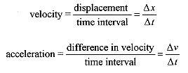
The motion of a particle (ballistic missiles, golf balls, and gas molecules are all examples of particles) is described by giving position, velocity, and acceleration usually as a function of time. For convenience in getting started we confine the discussion to one dimension. We also need to differentiate between distance and displacement, and speed and velocity.
If a dog fetching a stick runs in a straight line (the +x direction) 30m to pick up the stick and returns (the x direction) 26m then the total distance traveled is 56m but the displacement is +4m. Distance generally means total distance traveled while displacement is the actual difference between end point and beginning.
If the dog were to execute the fetching in 8s then the speed of the dog would be the total distance traveled divided by the time or 7m/s while the velocity, defined as the displacement divided by the time, would be 0.5m/s.
In a word equation form this is
The “ä” notation is read as “a change in” or “a small change in.”
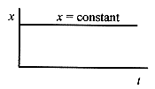
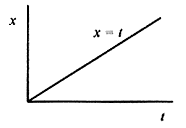
Let’s look at some simple relationships between position and velocity. Remember we are confined to one dimension. The simplest relation is x = constant. As shown in Fig. 2 1, the particle doesn’t move. There is no velocity or acceleration because x does not change with time. The first complication is x = t (Fig. 2 2). The particle moves equal increments in x in equal increments of time.
That is, the change in x from t = 1 to t = 2 is the same (same change) as when t goes from t = 2 to t = 3. The velocity then is a constant. And by definition the acceleration is zero.
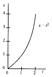
The next complication is x = t2. This graph is shown in Fig. 2–3. In this quadratic relationship, the simple definition of velocity begins to break down. Between t = 0 and t = 1 the velocity is (1 0)/(1 0) = 1. Between t = 1 and t = 2 the velocity is (4 1)/(2 1) = 3 and on and on with the velocity changing depending on the time interval chosen. Clearly the acceleration is not a constant. This velocity calculation fits our present definition and is equivalent to drawing a straight line between points on the smooth curve of x versus t.
Calculating velocity this way presents a problem because depending on the interval we will get different answers for the velocity. To find the velocity at t = 1, we found x at t = 1 and x at t = 2 and performed the velocity calculation. This is not a good approximation to the velocity at t = 1 because the average is between t = 1 and t = 2. A better approximation would be to take values of x between t = 1 and t = 1.1. Even better would be to take values between t = 0.99 and t = 1.01. And for even better approximations just shorten the time interval centered about t = 1. As the interval gets smaller we will get a better and better measure of velocity. In Fig. 2–4 the slope of the straight line from x = 1 to x = 4 represents the average velocity between x = 1 and x = 4. The slope of the straight line tangent to the curve at x = 1 represents the velocity at x = 1. Instantaneous Velocity and Acceleration A more versatile definition of velocity is äx/ät, where the interval ät is very small and centered about the time where the velocity is desired. This approach leads to a general method for obtaining an expression for velocity that can be evaluated at any point rather than going through the numeric calculation whenever we want a velocity.
In words, this definition is stated as the instantaneous velocity which is the value of äx/ät as ät approaches zero. In equation form this is written as
This definition of the derivative as the limit of äx/ät as ät approaches zero is the slope of the tangent to the curve evaluated at the point in question. Thus if we want to find the velocity of any particle traveling according to a polynomial relation between x and t all we need is a general technique for finding the slope of the tangent to the polynomial at any point.
The instantaneous acceleration is defined as the value of äv/ät as ät approaches zero. In equation form this is
The instantaneous acceleration is the slope of the tangent to the curve of v versus t.
The general expression for the slope of any polynomial is discussed in the Introduction, Mathematical Background. For a polynomial of the form x = ctn the expression for the slope at any point is cntn 1. Stating this in calculus terms; for any function x = ctn, the derivative of the function is cntn 1. This can be verified in the case of the parabola by taking successively smaller intervals of ät and äx at any point t to verify that the slope at any point is 2t.
Kinematic Equations of Motion.
The kinematic equations of motion are derived under the assumption of constant acceleration. While this may at first seem to be a restriction, there are a large number of problems where the acceleration is a constant. The simplest and most obvious are falling body problems, that is, problems involving bodies falling on (or near) the surface of the earth where the acceleration due to gravity is a constant. Falling body problems are taken up in a separate chapter. In the derivation of the kinematic equations of motion a good image to keep in mind is that of falling bodies
Starting with the assumption of constant acceleration we can write
which can be rearranged to vf = v0 at.
Usually the f subscript is dropped to read v = v0 + at.
and further substituting for v = v0 + at. we arrive at x = x0 + v0t + (1/2)at2.
and upon rearranging
Summarizing, these four kinematic equations of motion are written as
The first three equations relate displacement, velocity, and acceleration in terms of time while the fourth equation does not contain the time.
Now let’s apply these four equations to some typical problems. Remember that the kinematic equations of motion allow us to describe the position, velocity, and acceleration of a mass point.
2 1 A train starts from rest (at position zero) and moves with constant acceleration. On first observation the velocity is 20m/s and 80s later the velocity is 60m/s. At 80s, calculate the position, average velocity, and the constant acceleration over the interval.
Solution: Diagram the problem.
If the acceleration is constant then the average velocity is the average of 20m/s and 60m/s, or 40m/s, and at an average velocity of 40m/s and 80s, the distance traveled is 3200m.
2-2 For the situation of problem 2-1, calculate the position of the train at 20s
2–3 For the situation of problem 2-1 find the time required for the train to reach 100m
This is a quadratic equation in t. Without units the equation is
 and has solutionsThe negative answer is inappropriate for this problem so take t = 4.5s.
2–4 For the situation of problem 2 1 find the velocity of the train at 120m.
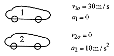
2–5 Two vehicles are at position x = 0 at t = 0. Vehicle 1 is moving at constant velocity of 30m/s. Vehicle 2, starting from rest, has acceleration of 10m/s2. A typical question of this situation is “Where do they pass?”
Solution: First diagram the situation.
The question “Where do they pass?” translated into algebra means “What is the value of x when they pass?” This can be determined by writing equations for the position of each vehicle and
Setting x1 = x2 gives the time when they pass as 30t = 5t(t 6) = 0; so the vehicles pass at t = 0 and t = 6. Putting t = 6s in either equation for x (x1 or x2) gives 180m as the distance.
2–6 For the situation in problem 2–5, when do the vehicles have the same velocity?
Solution: In algebra this means to set the equations for velocity equal (v1 = v2) and solve for the time. Remember that three of the four equations of motion are functions of time so most question are answered by first calculating the time for a certain condition to occur.
Now that we know when, we can calculate where they have the same velocity. Use either equation for position and t = 3.0s
2–7 For the situation of problem 2–5. what is the position, velocity, and acceleration of each vehicle when vehicle 2 has traveled twice the distance of vehicle 1?
Solution: The time when this occurs is when x2 = 2×1: 5t2 = 60t or 5t(t – 12) = 0
This gives times of t = 0 and t = 12. The time t = 0 is correct, though uninteresting. The time t = 12 is the physically interesting answer.
At t = 12:
From the original statement of the problem, v1 = v10 = 30m/s and a1 = 0.
Now solve for the remaining variables for the second vehicle by substitution
From the original statement of the problem a2 = 10m/s.
2–8 Two trains are traveling along a straight track, one behind the other. The first train is traveling at 12m/s. The second train, approaching from the rear, is traveling at 20m/s. When the second train is 200m behind the first, the operator applies the brakes producing a constant deceleration of 0.20m/s2. Will the trains collide, and if so where and when?
Solution: First, diagram the situation. Our strategy will be to write down the equations for each train using equations (2 1) through (2–6) and the information provided in the problem. Take t = 0 when the brakes are applied and the first train is 200m ahead of the second. This makes the position of the first train 200m at t = 0 (x10 in equation 2 2).
The question as to whether the trains collide means: “Is there a real (time) solution to the equation resulting from setting x1 = x2.
If there are no real solutions to this equation then the trains do not collide. Drop the units and write 0.10t2 8t + 200 = 0 which is solved by quadratic formula
Since there are no real solutions to this equation there are no times when the trains collide.
<><><><><><><><><><><><>
2–9 Change problem 2–8 by giving the second train an initial velocity of 25m/s. This will give a real time for the collision. Find the collision time.
Solution: The situation is now as shown in the Fig. 2–8.
Again setting the expressions for x1 and x2 equal and dropping the units produces 200 + 12t = 25t 0.10t2 or 0.10t2 13t + 200 = 0 with solutions
The two times correspond to when x1 = x2. The earliest time is the first coincidence and the end of the (physical) problem. The position at this time can be obtained from either expression for x.
Verify this distance by using x2.
The velocity of the second train at collision is
The relative velocity (between the two trains) is v = 1.4m/s.
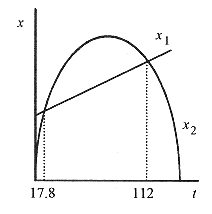
The two times are the result of the quadratic in t. The two solutions occur when the curves cross. The equation for x1 = 200 + 12t is a straight line of slope 12 starting at 200. The equation for x2 = 25t 0.10t2 is a parabola that opens down. Figure 2–9 (not to scale) shows the two curves.
While the “mathematics” produces two times, the reality of the problem dictates the earlier time as the one for the “collision.”

