Simulation Results
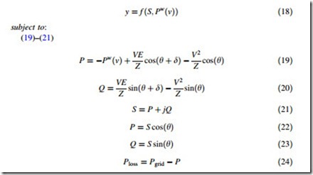
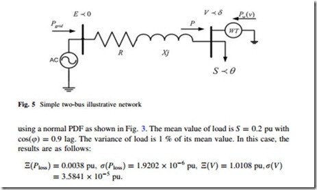
The introduced approaches are implemented in GAMS [38] environment solved by CONOPT solver running on an Intel® CoreTM2 Duo Processor T5300 (1.73 GHz) PC with 1 GB RAM. In order to illustrate the concept of each introduced uncertainty modeling method, a simple two-bus network is used as shown in Fig. 5. A load is fed by a wind turbine (WT) and through a feeder with the impedance of Z ¼ R þ jXðXÞ. The apparent power of load is L ¼ S -< h ¼ SðcosðhÞþ j cosðhÞÞ. It is assumed that the magnitude of load (S) is uncertain. Another uncertain parameter is the power generation of WT. The rated capacity of wind turbine is 0.1 pu.
The impedance of the line is Z\h ¼ 0:2667\1:0717 pu. The sending end voltage is kept constant as E = 1.05 pu. The mean value of load is S = 0.2 pu with cos(u) = 0.9 lag.
The function f can be defined based on the requirement of the decision maker. It can be active losses, voltage magnitude at load bus, etc.
In case there is no uncertainty about the load value and assuming zero power injection by WT, the problem is solved and the values of unknown variables are found to be as follows: V = 1.006 pu, d = -0.029 Rad, Ploss ¼ 0:005 pu,
Pgrid ¼ 0:185 pu. The scale parameter of Rayleigh PDF for wind speed is 8, respectively.
Monte Carlo Simulation
In this section, it is assumed that the wind generation is dependent on wind speed as described in Sect. 3.1. The uncertainty of load is modeled probabilistically
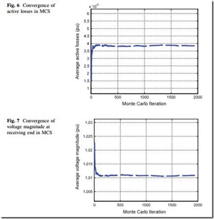
The stopping criteria is defined as the maximum number of iterations that should not exceed 2000. This number chosen is arbitrary, however, it is a typical choice for the maximum number of MCS iterations. It can be observed in Figs. 6 and 7 that the expected values of uncertain parameters are converged in iteration 1000.
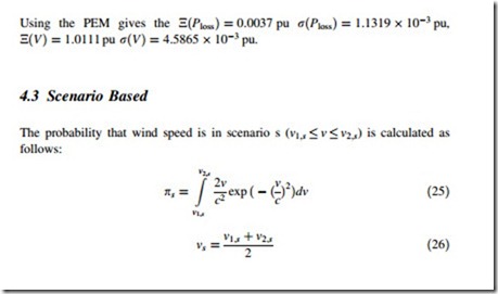
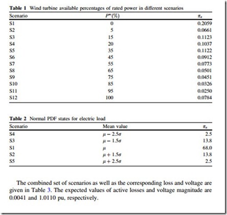
where v1;s; v2;s are the limits of wind speed’s interval in states. The generated power of wind turbine in states is calculated using the obtained vs and (12). The percentages of producible wind power in each scenario are given in Table 1.
In order to cover the whole wind speed variation range, 12 different scenarios are considered in this study. The scenario s1 refers to the case where the wind
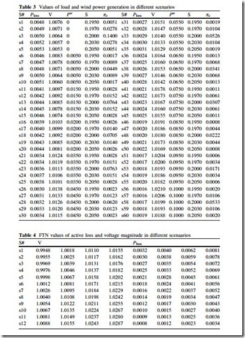
The combined set of scenarios as well as the corresponding loss and voltage are given in Table 3. The expected values of active losses and voltage magnitude are 0.0041 and 1.0110 pu, respectively.
Hybrid Case
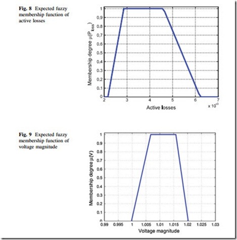
In this case, it is assumed that the PDF of wind speed is available, however, no historic data is at hand for load values. This situation can be handled using the fuzzy arithmetic and expert opinion regarding the membership function of load. The expert gives the following trapezoidal fuzzy number for describing the nature of uncertainty. S = (0.16, 0.18, 0.22, 0.25). Using the introduced technique in Sects. 2.3 and 3.3, the problem described in (14) is solved for each scenario and the components of output’s TFN are calculated. The FTN values of active loss and voltage magnitude in different scenarios are given in Table 4. The expected fuzzy membership function of active losses and voltage magnitude are shown in Figs. 8 and 9, respectively.
The crisp values of active loss and voltage magnitude are 0.0042 and 1.0105 pu, respectively. In order to have a better understanding of the obtained results, the expected values of active loss and voltage magnitude given by different methods
Table 3 Values of load and wind power generation in different scenarios
are described in Table 5, although the case analyzed in hybrid method is inherently different from the first three ones. In the first three stochastic cases, the value of load was described using a probabilistic method. It did not hold for the hybrid case. In this case, the load was described using a fuzzy membership function. Obviously the computational burden of hybrid case is higher than scenario based approach since it needs to run two optimizations in each a level. In this simulation, just two a levels are considered (a = 0, 1) so four optimizations are needed to obtain the final solution.
